Abstract
Main topic discussed in this paper is the practical
application of image processing systems, particularly those resolving the
problem of image restoration from 2D slices, which are acquired via CCD cameras
connected to various types of optical devices and subsequently processed by
computer.
Keywords: convolution, objective,
numerical
aperture, in-focus plane,
out-of-focus plane, inverse filtering, PSF.
1. Introduction
The human being is not able to handle all of the
received information. The information obtained at the very first stages of
human observation of the real world is always accompanied by, according to
previous sentence, 'surplus' data. The area of image preprocessing serves as
instrument for suppressing such undesirable features of image, which is
sometimes equal to emphasizing the desired ones either by empirical or
theoretical methods. Thereinafter we focus on describing some image
preprocessing techniques.
We begin with listing of several image-depreciating
effects:
·
glare and shading of
objects
·
blurring
·
3D to 2D space
projection
·
limited resolution of
devices
·
additive and multiplicative
noise
·
radiation induced by
examined object
·
motion of object
Very often an image
contains much more information than can be perceived. Details are invisible due
to noise or other obstacles. Some of image degradations are introduced by human
factor. This includes improperly focused optical devices, construction defects
etc. Our intention is to describe some of them and to try to eliminate their
influence on the image. This can be achieved by using of explicit information
about optical devices.
2. Image
reconstruction techniques
"Renovation" is
an image preprocessing technique, which tries to reduce the image defects by
procedures based upon estimation of defect characteristics. While it is obvious
that reconstructed image is merely an approximation of the original, the goal
is to minimize the differences. Considering the viewpoint from which solution
arises, we can split image reconstruction techniques into deterministic and
stochastic. Deterministic techniques are only suitable for image that contains
none or irrelevant amount of noise. The reconstructed image is a result of
applying the inverse transformation to the acquired image (i.e. the image
obtained by a physical device). On the other hand stochastic methods are based
upon starting estimation of original image and successive iteration which must
satisfy convergence condition. However, in both cases it is essential to have
the degrading transformation properly modeled.
Considering the type of availability of
information, we recognize a priori
and a posteriori information. A priori knowledge can be obtained e.g.
during scanning of moving objects. In such cases ablation of defects (motion
blur) can be accomplished using information about such physical parameters as
direction and speed of movement. Defects detected during image analysis are
considered a posteriori.
2.1.
Image reconstruction where the degrading transformation is known
In order to solve the
problem of reducing the image defects we firstly are obligated to formally
describe the process of degradation. This can be done by following formula
g(x,y)
= s![]() + v(x,y), (1)
+ v(x,y), (1)
where g(x,y) represents resulting image, f(x,y)
the original image, s - nonlinear function, v(x,y) the noise. This model is
often simplified, neglecting nonlinearity of s(x,y) and constraining h(x,y,a,b)
to the time-invariant convolutional core, which is used to describe the defects
of the optical device. Simplified formula
g(x,y) = f(x,y) Ä h(x,y) + v(x,y), (2)
represents the fundament for image restoration algorithms. The design
of h(x,y) called Point Spread Function will be explained in details later in
the paper.
Objective lens of device is focused on small
area of examined specimen. However acquired image contains light from non-focal
sources. As a result of this effect, image information coming from in-focus
plane is fairly blurred by light diffraction. While PSF was defined for both
in-focus and out-of-focus plane we are able to calculate resulting image by
summing the convolution of in-focus data with in-focus PSF and the convolution
of out-of-focus data with out-of-focus PSF. Let us consider simple case, when
merely two out-of-focus planes contribute to blurring of the image from
in-focus plane [Agar89]:
g![]() (x,y)
(x,y)![]() f
f![]() (x,y)
(x,y)![]() h
h![]() (x,y)+f
(x,y)+f![]() (x,y)
(x,y)![]() h
h![]() (x,y) +f
(x,y) +f![]() (x,y)
(x,y)![]() h
h![]() (x,y), (3)
(x,y), (3)
where functions f![]() (x,y), f
(x,y), f![]() (x,y), f
(x,y), f![]() (x,y) are actual images.
Functions h
(x,y) are actual images.
Functions h![]() (x,y), h
(x,y), h![]() (x,y), h
(x,y), h![]() (x,y) are in-focus and
out-of-focus PSF. As the actual image data from individual planes are unknown,
we will use their approximation. Hence g
(x,y) are in-focus and
out-of-focus PSF. As the actual image data from individual planes are unknown,
we will use their approximation. Hence g![]() (x,y)
(x,y) ![]() f
f![]() (x,y) and g
(x,y) and g![]() (x,y)
(x,y) ![]() f
f![]() (x,y). Therefore data from
in-focus plane can be calculated using modified equation
(x,y). Therefore data from
in-focus plane can be calculated using modified equation
f![]() (x,y)
(x,y)![]() (g
(g![]() (x,y)-c.(g
(x,y)-c.(g![]() (x,y)
(x,y)![]() h
h![]() (x,y)+ g
(x,y)+ g![]() (x,y)
(x,y)![]() h
h![]() (x,y)))
(x,y))) ![]() h(x,y), (4)
h(x,y), (4)
where constant c is determined empirically,
function h(x,y) describes filter for in-focus plane. This process is also
called nearest-neighbours algorithm [Agar89].
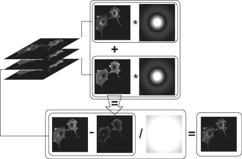
Figure
1: Scheme of the nearest-neighbours algorithm with two out-of-focus planes,
using CTF unction, meanwhile the
Fourier transformation is applied to each slice
By modification of this procedure we obtain
no-neighbours algorithm [Monck92]
f![]() (x,y)
(x,y) ![]() (g
(g![]() (x,y)-c.(g
(x,y)-c.(g![]() (x,y)
(x,y)![]() h
h![]() (x,y) +g
(x,y) +g![]() (x,y)
(x,y)![]() h
h![]() (x,y)))
(x,y))) ![]() h(x,y), (5)
h(x,y), (5)
assuming that f![]() (x,y)
(x,y) ![]() g
g![]() (x,y) and f
(x,y) and f![]() (x,y)
(x,y) ![]() g
g![]() (x,y).
(x,y).
2.1.1.
Non-iterative methods of inverse filtering
Techniques of inverse filtration are derived
from basic model defined by (2). For effective applying of inverse filtration
the assumption of minimal noise is necessary.
Further we take advance (in terms of
calculation) of fact, that convolution can be calculated as multiplication in
spectral domain (i.e. after applying of DFT):
G(u,v) = F(u,v).H(u,v) + V(u,v) (6)
We can obtain the original image by filtering
with a function inverse to H(x,y):
F(u,v) = G(u,v).H![]() (u,v) – V(u,v).H
(u,v) – V(u,v).H![]() (u,v) (7)
(u,v) (7)
In cases when noise is relevant, it appears
in equation (7) as an additive error, which has its maximal amplitudes mostly
in higher frequencies of the spectrum. By neglecting noise we obtain:
![]() (u,v) = G(u,v).H
(u,v) = G(u,v).H![]() (u,v) (8)
(u,v) (8)
Afterwards we apply linear operator Q to the
F to improve the flexibility of the found approximation. Our task is to find
the minimum of J(F) using the method of Lagrange multipliers.
J(![]() ) =
) =  +
+ ![]() .(
.(![]() ), (9)
), (9)
where ![]() is Lagrange
multiplier.
is Lagrange
multiplier.
![]() =
=![]()
![]() .G(u,v), (10)
.G(u,v), (10)
Equation (10) serves as a base for finding
suitable linear operator Q and successive determination of g. Well-known Wiener filter is often used.
Estimation of statistical properties of image noise is a criterion for the
choice of the most appropriate operator.
![]()
![]()
 .G(u,v), (11)
where k is obtained empirically.
2.1.2.
Iterative methods of inverse filtering
Principal idea of iterative procedures used
in inverse filtration is to estimate and gradually improve the quality of
approximation of the original image. To minimize the distance of related images
is one of the possibilities. Let us use following relation between the original
and measured image
g(x,y)
= f(x,y) Ä h(x,y), (12)
D![]() (x,y) =
(x,y) = ![]() (13)
(13)
D![]() (x,y) is the measure of
quality of estimation in the k-th step of iteration. o
(x,y) is the measure of
quality of estimation in the k-th step of iteration. o![]() (x,y) - represents the
approximation of f(x,y) in the k-th step of iteration. In terms of previous
formula we have to minimize D
(x,y) - represents the
approximation of f(x,y) in the k-th step of iteration. In terms of previous
formula we have to minimize D![]() (x,y). Now we define the
k-th step of iteration as
(x,y). Now we define the
k-th step of iteration as
o![]() (x,y) = o
(x,y) = o![]() (x,y).w
(x,y).w![]() (x,y), (14)
(x,y), (14)
where w![]() is vector of correction.
Choice of suitable correction vector is necessary. We notice some well-known
proposals of the correction vector:
is vector of correction.
Choice of suitable correction vector is necessary. We notice some well-known
proposals of the correction vector:
·
Jansson & van Cittert
w![]() (x,y) = 1 +
(x,y) = 1 + ![]() .
.![]() .( g(x,y) - (h(x,y)
.( g(x,y) - (h(x,y)![]() o
o![]() (x,y)) ) (15)
(x,y)) ) (15)
·
Meinel
w![]() (x,y) =
(x,y) = ![]() (16)
(16)
·
Richardson & Lucy
w![]() (x,y) = h(x,y)
(x,y) = h(x,y)![]() (
(![]() ) (17)
) (17)
Aforementioned methods can be extended with possibility of noise reduction so that in each step of iteration we apply Gaussian filter to the processed image. Hence modified Meinel's algorithm is:
w![]() (x,y) = L
(x,y) = L![]() (x,y)
(x,y)![]()
![]() (18)
(18)
The formulae listed above belong to very
repeatedly used in the field of image preprocessing. h(x,y) is called Point
Spread Function.
3. Point Spread Function
Degradation and blurring of optically
acquired image is described via PSF. PSF is a mathematical description of how
the points from an out-of-focus plane are transformed to the measured image.
Hence this function is individual for each optical device, depends on object
glass used and is influenced by numerical aperture, by errors and aberrance of
the used lenses and by index of refraction of used immerse media. PSF is an
approximation of theoretical PSF and it is obtained either considering
aforementioned physical parameters in theoretical optics model or can be
measured empirically.
3.1. Theoretical
approach
Image degradation effect can be computed as
an approximation of the original function with aid of theoretical optics. There
exists numerous methods of simulating PSF; they mostly arise from the basic
theoretical model described in works of Castleman [Cast79] and Agard [Agar84].
Theoretical PSF is considerably different than real PSF in the way that it
represents ideal model of optical devices and it is not able to fully describe
the variations of physical parameters of practically used optical devices. In
spite of that we can reach very substantial image improvements. PSF is modeled
via CTF, which is its equivalent in frequency domain.
CTF depends on physical parameters of optical
device, such as:
·
numerical aperture
·
refractive index of medium
·
x/y-dimension of pixel
·
image size
·
wavelength of emitted light
S(q)=![]() (2b - sin 2b)jinc[
(2b - sin 2b)jinc[![]() (1 –
(1 – ![]() )
)![]() ], (19)
], (19)
where q = ![]() ,
,
jinc(x) = 2J1(x) / x ,
and J1(x)
is Bessel function. This function is usually
included in the math library of a C language compiler.
b = cos-1 (![]() ) ,
) ,
w = - df - Dz cos a + (df2 + 2dfDz + Dz2cos2 a)![]() ,
,
where d![]() is focal distance of the objective lens in micrometers and Dz is distance from in-focus plane in micrometers. From
(19) follows that planes equally distant from out-of-focus planes are
equivalent.
is focal distance of the objective lens in micrometers and Dz is distance from in-focus plane in micrometers. From
(19) follows that planes equally distant from out-of-focus planes are
equivalent.
a = sin-1(NA / h),
Parameter a is
the widest angle of incident light rays, relative to the optical axis, that can
be captured by the objective lens. NA is the stated numerical aperture on the
objective lens and h is
the index of refraction of the immersion medium recommend by the manufacturer
of the objective lens.
fc = 2 NA / l = 2 h sin a / l ,
where fc is the inverse of the
resolution limit, which is the highest spatial frequency that can be passed by
the objective. Parameter l is the wavelength of emission light.
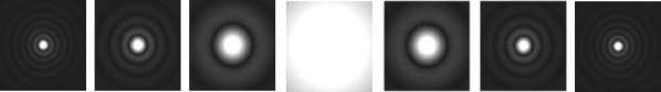
Figure 2: CTF NA=1.4, df =800 mm, h = 1.515, Xdim = 0.295858 mm, Ydim = 0.295858 mm, distance of defocus 1 mm, l = 0.488 mm
3.2. Empirical approach
In various cases of reconstruction of
depreciated display image it is satisfactory to know PSF as an abstract approximation
of the original PSF, but in some other cases, as the aberrance and others
anomalies of individually used lenses bring about cancellation of image, that
we cannot abolish by present approximation, it is necessary to obtain PSF by an
empirical manner. We can define PSF as a transformation of a light emitting
point, whose magnitude is smaller than resolution of the optical system, so we
chose a point light source for examined object. Measuring out these image
parameters yields PSF, that itself more approaches to original. If the optical
system does not contain any anomalies (so we can discuss ideal optical device),
then examined point shows itself as a luminous spot (appearing at display image
as a pixel) at in-focus plane, while there are no spots at out-of-focus planes.
At factual conditions the light emitting point appears as a circular
aggregation of light spots, with fading intensity depending on the radius.
Circular aggregation increases in radius with clearance of in-focus plains.
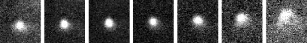
Figure
3: Empirical PSF
4. Future work
Work presented in this paper provides compact
tool for processing of image obtained via CCD camera connected to optical
devices. Algorithms use either theoretical or empirically measured
approximation of point spread function. Merely small number of physical
parameters is considered in existing models of point spread function.
Considering more parameters there appears the possibility of more accurate
modeling of point spread function for individual optical systems. This seems to
be vast and very rich field, which offers amount of opportunities for research.
5. Conclusion
The aim of this work was to collect various
methods of image preprocessing, their improving and implementation. These
techniques try to give human instruments for better understanding, storage and
further processing of acquired images.
6. Acknowledgements
We
would like to thank Dušan Chorvát for fruitfull discussions, for his support
and assistance during experiments. We also appreciate material support from
International Laser Center in Bratislava.
References:
[Gonz87]
Gonzales R.C., Wintz P.: Digital Image
Processing, Addison-Wesley, Mass., 1987
[Ruži95]
Ružický E. , Ferko A. : Počítačová
grafika a spracovanie obrazu, Sapienta, Bratislava, 1995
[Šonk92]
Šonka M. , Hlaváč V. : Počítačové videní,
GRADA, Praha, 1992
[Agar84]
Agard D. A. : Optical sectioning
microscopy: Cellular architecture in tree dimensions,
Annu.Rev.Biophys.Bioeng, 1984
[Cast79]
Castelman K. R. : Digital Image
Processing, Englewood Cliffs, New Jersey: Prentice-Hall, 1979
[Monc92]
Monck J. R. , Oberhauser A. F. et al.: Thin-section
ratiometric Ca![]() images obtained by optical sectioning of fura-2 loaded mast
cells, J.Cell Biol., 1992
images obtained by optical sectioning of fura-2 loaded mast
cells, J.Cell Biol., 1992
[Keat99] Keating J. , Cork R. J. : Improved Spatial Resolution in Ratio Images
Using Computational Confocal Techniques, A Practical Guide to the Study of
Calcium in Living Cells, Volume 40 of Methods in Cell Biology, Academic Press,
1999