Introduction

In image processing it is a fundamental problem how to reconstruct features (like the original gradients) from sampled data. A typical example is the reconstruction of medical data obtained as CT or MRI scans. The data can be sampled at regular or irregular grids points. If we use direct volume rendering to visualize such a data set staircase artifacts can occur. In case of binary segmented data the staircase aliasing is stronger than in case of gray-scale data, where the gradients can be estimated more accurately. A binary volume can be obtained as a result of a segmentation. The segmented data cannot be rendered directly, because the result looks like built from Lego pieces. Therefore, various preprocessing techniques are used to eliminate this aliasing. The classical method is convolution-based filtering. Convolution-based methods have mostly local influence, because of the limited support of the kernel function. Although filtering with a wide kernel causes dependency on wider neighborhood, it is rather time-consuming and removes fine details. There are several approaches for solving this problem. One research direction is interpolation oriented assuming, that accurate samples are available. The sinc and cosc functions are considered as ideal interpolation and derivative filters respectively. These derivative reconstruction techniques based on windowing are local methods as for practical reasons only a limited number of neighboring samples are taken into account. Another approach for derivative reconstruction is approximation oriented. Here it is assumed, that the sampled function is noisy, which is typical, when some real physical properties are measured. The basic idea is to estimate the inclination or the normal from a larger neighborhood. In order to reduce staircase aliasing, several methods were proposed for normal computation especially in binary volumes. Contextual shading techniques try to fit locally approximated plane or a biquadratic functions to the set of points that belong to the same iso-surface. These methods are time consuming and limited to a certain neighborhood. A rather new research direction is based on a gradient estimation using 3D distance maps. The new method we have implemented, designed by Neumann et al. 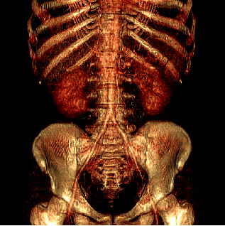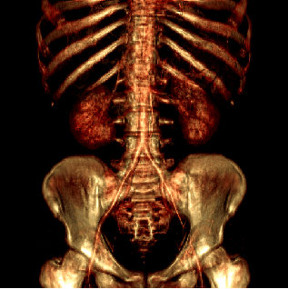[4] is a general tool for filtering binary and gray-scale data sets. Figure 1 illustrates this filtering technique on a CT scan of a human body.

Figure 1: Direct volume rendering of a human body using the original (a) and the filtered (S = 1, G = 1) data (b).

(a)	(b)

Similarly to the distance maps, generated from binary volumes, this filtering technique creates a smooth volume from gray-scale data. Unlike convolution based filtering, the smoothing effect is global due to a global curvature minimization. Feature preservation is the main characteristic of this novel filtering approach. By globally penalizing large gradient deviations, important features and fine details like edges or iso-surfaces are preserved. The method is based on a quadratic penalty function $E$. $E$ is defined so that feature preservation and smoothing is simultaneously possible. Therefore $E$ consists of the following three components summed over every sample point $i$:

• difference squared between filtered value $\tilde{f}_{i}$ and original value $f_{i}$
• difference squared between the gradient of the filtered value $\tilde{%f}_{i}$ and the original value $f_{i}$
• the squared curvature of the filtered function $\tilde{f}$

The 1D case of the penalty function $E$ has the following structure:

$$E=\sum_{i}[(\tilde{f}_{i}-f_{i})^{2}+G\cdot[(\tilde{f}_{i+1... ...\cdot(\tilde{f}_{i+1}+\tilde{f}_{i-1}-2 \tilde{f}_{i})^{2}].$$ (1)

The weights $S$ and $G$ determine the relative importance of feature preservation as opposed to smoothing. At the minimum location of the penalty function $E$ the partial derivatives according to all the $N$ unknown values $\tilde{f}_i$ have to be equal to zero, where i = 0, 1, 2, ..., N-1:

$$\partial E(\tilde{f}_0, \tilde{f}_1, \tilde{f}_2, ..., \tilde{f}_{N-1}) / \partial \tilde{f}_i = 0.$$ (2)

As penalty function $E$ is a quadratic function, the partial derivatives are linear functions of variables $\tilde{f}_i$. Therefore, having all of these partial derivatives evaluated, a large linear equation system is obtained with $N$ unknown variables:

$$A\cdot\tilde{f}=m,$$ (3)

where $A$ is a sparse coefficient matrix, and $\tilde{f}$ is the unknown vector containing the $N$ samples of the filtered function. Vector $m$ is derived from the original function samples $f_{i}$ in the following way:

$$m_{i}=f_{i}-2G\cdot(g_{i+1}-g_{i-1}).$$ (4)

Matrix $A$, derived from the partial derivatives, is a band matrix defined by a symmetric point spread vector $p$:

$$p = [p_1,p_2,p_3,p_4,p_5] = [S-G, -4S, 1 + 6S + 2G, -4S, S-G],$$ (5)

$$A = \left[ \begin{array}{cccccccc} p_3 & p_4 & p_5 & 0 & ... ...\\ 0 & 0 & 0 & 0 & p_1 & p_2 & p_3 & \end{array} \right].$$

In fact, the multiplication of $\tilde{f}$ with coefficient matrix $A$ is a convolution of the unknown vector $\tilde{f}$ with kernel $p$. Therefore, it is not necessary to use any computationally expensive linear algebra method, since a simple deconvolution leads to the solution. Such a deconvolution can be efficiently performed in frequency domain. Using fast Fourier transformation, the filtering algorithm consists of the following steps:

1. estimation of gradients $g_{i}$ using linear regression
2. non-linear operations on the gradient function $g$
3. calculation of function $m$ using the modified $g$
4. $M=FFT(m)$ - Fourier transformation of function $m$
5. $P=FFT(p)$ - Fourier transformation of function $p$
6. $\tilde{F}=M/P$ - deconvolution in frequency domain
7. $\tilde{f}=INVFFT(\tilde{F})$ - inverse Fourier transformation of $\tilde{F}$