Volume rendering

Figure 5: Volume visualisation using transparent elements

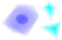Although drawing well-selected surfaces is extremely useful, there are also various techniques to render the volume of objects. These make extensive use of transparency to give an impression of value distribution. Values are coded as the opacity of the media, resulting in an X-ray like image. Usually, volumes are rendered with the use of particle systems or volume tracing. However, in case of finite element data, these time-consuming methods may be substituted with a simpler one if we render elements one by one. Assuming that the value we are to display is constant in each element, a single more-or-less transparent simplex is not extremely hard to draw. Within the polygonal segments formed by overlapping front and back facets the thickness of the material, and so its opacity changes linearly. These polygons should be rendered beginning form the furthest element, with appropriate opacity values assigned to the vertices. Naturally, these values, and the vertices themselves depend on the viewing angle, and so the polygons have to be recalculated for every new camera vector. Unfortunately, the method fails as soon as the value within an element is not constant, because the opacity does not change linearly then.