Fig. 8: Definition of shell. Leading curve and axis (identical) are black, distance function (visualized as rotated curve) is gray.
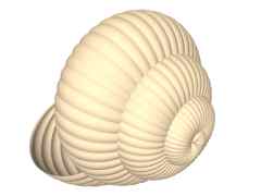
Fig. 9: A shell.
Enough of theory, lets make some practical examples. Creation of pictures is made in two steps. As a first step, objects' meshes are produced with package libgro (http://libgro.sourceforge.net). Visualization itself is done in Persistence of Vision raytracer (http://www.povray.org). Software package libgro is part of my master's thesis Generalized Rotational Objects. Thesis is available online via URL http://dw.cech.cjb.net.
Lofted variant of generalized solid of revolution with distance function is well suited to model shell that would many snails envy. In fact, shell is only a modified cone. The only axis has both x and y coordinates constant and zero. This way it is identical to leading curve, that goes directly through the center of cone. Leading curve has spiral shape. Distance function is simple linear falloff from one to zero with three-percent modulation to make rings. The exact definition is summed in table 1 and shown in figure 8. Resulting image is shown in figure 9.
| Curve/function | Definition |
|---|---|
| Leading curve | x=t.cos(8πt) y=t.sin(8πt) z=2(1-cos(0.5πt)) |
| Axis | x=0 y=0 |
| Distance function | t(0.97+0.03sin(173.2πt)) |
|
Fig. 8: Definition of shell. Leading curve and axis (identical) are black, distance function (visualized as rotated curve) is gray. |
Fig. 9: A shell. |
Both square and circle can be created using only one axis (with Manhattan metrics in case of square and Euclidean in case of circle). Unfortunately, one axis cannot have more than one metrics assigned. We need to use little trick - two spatially identical axes, that differs only with metrics and weight. Along axes, a linear blend of weights is created. While "Manhattan" one's weight fades out (from one to zero), "Euclidean" one's weight fades in (from zero to one). Sum of both weights is one in each point of axes. Rest of definition is simple. Leading curve is identical to axes and distance function is constant (any positive value does the job fine). The final image is shown in figure 4.