A Framework for Flexible, Hardware-Accelerated, and

High-Quality Volume Rendering

VRVis Research Center for Virtual Reality and Visualization
Vienna / Austria
http://www.VRVis.at/vis/

Abstract

Through the invention of new rendering algorithms and an enormous development of graphics hardware in the past it is now possible to perform interactive hardware-accelerated high quality volume rendering as well as iso-surface reconstruction on low cost standard PC graphics hardware.
In this paper we introduce a flexible framework that supports the most common graphics adapters without additional need of setup as well as several vendor-dependent OpenGL-extensions like pixel-, texture- and fragment-shader. Additionally the framework integrates most recent presented rendering techniques which significantly improve image-quality as well as performance of standard hardware based volume rendering (and iso-surface reconstruction) approaches.
Special focus of the presented framework is concentrated on splitting up the rendering process into several principal subtasks to provide easy reuse possibilities by only extending the appropriate modules without need to change the overall rendering implementation.
The major objective of the prototype is to provide comparison possibilities for several hardware accelerated volume visualizations with respect to performance and quality.

Keywords: volume rendering, volume visualization, graphics hardware, isosurface-reconstruction, OpenGL, flexible framework

1 Introduction

For visualization of volumetric data direct volume rendering [6,7] is an important technique to get insight into data. The key advantage of direct volume rendering over surface rendering approaches is the potential to show the structure of the value distribution throughout the volume. Due to the fact that each volume sample contribution to the final image is included, it is a challenge to convey that value distribution simple and precisely.
Because of an enormous development of low-cost 3D hardware accelerators in the last few years the features supported by consumer-oriented graphics boards are also very interesting for professional graphics developers. Especially NVIDIA's [15] pixel- and texture shader and ATI's [13] fragment shader are powerful extensions to standard 2D and 3D texture mapping capabilities. Therefore high-performance and high-quality volume rendering at very low costs is now possible. Several approaches of hardware-accelerated direct volume rendering have been introduced to improve rendering speed and accuracy of visualization algorithms. Thus it is possible to provide interactive volume rendering on standard PC platforms and not only on special-purpose hardware.
In this paper we present an application that includes several different visualization algorithms for direct volume rendering as well as direct iso-surface rendering. The major objective of the prototype is to provide comparison possibilities for several hardware accelerated volume visualizations with respect to performance and quality. On startup of the software, the installed graphics adapter is detected automatically and regarding to the supported OpenGL-features the user can switch between the available rendering modes supported by the current graphics hardware. The full functionality includes pre- and post classification modes as well as pre-integrated classification modes (see Section 3.2 and 3.3). All algorithms are implemented exploiting both 2D or 3D texture mapping as well as optional diffuse and specular lighting. Additionally we have adopted the high-quality reconstruction technique based on PC-hardware, introduced by Hadwiger et al. [4], to enhance the rendering quality through high-quality filtering.
The major challenge is combining diverse approaches in one simple understandable framework that supports several graphics adapters which have to be programmed completely different and still provide portability for implementation of new algorithms and support of new hardware-features.
The paper is structured as follows. Section 2 gives a short overview of work that has been done on volume rendering and especially on hardware-accelerated methods. Section 3 is then going to introduce the main topic, namely volume rendering in hardware (texture based), providing a brief overview of the major approaches and describing different classification techniques. In Section 4 we will then discuss the implementation in detail, starting with the basic structure of our framework, afterwards describing the differences between ATI and NVIDIA graphics adapters and the implementation of several volume rendering techniques as well as iso-surface reconstruction modes. This section also covers some problems that have to be overcome if supporting graphics adapters from different vendors. Moreover the section includes some performance issues and other application specific problems we encountered during prototype implementation. Section 5 summarizes what we have presented and additionally some future work that we are planning at the moment will be briefly mentioned.

2 Related Work

Usually visualization approaches for scalar volume data can be classified into indirect volume rendering, such as iso-surface reconstruction, and direct volume rendering techniques that immediately display the voxel data.
In contrast to indirect volume rendering, where an intermediate representation through surface extraction methods (e.g. the Marching Cube algorithm [8]) is generated and then displayed, direct volume rendering uses the original data. The basic idea of using object-aligned slices to substitute trilinear by bilinear interpolation was introduced by Lacroute and Levoy [5], the ShearWarp algorithm.
The texture-based approach presented by Cabral [2] has been expanded by Westermann and Ertl [16], who store density values and corresponding gradients in texture memory and exploit OpenGL extensions for unshaded volume rendering and shaded iso-surface rendering. Based on their implementation, Meißner et al. [10] have extended the method to enable diffuse illumination for semi-transparent volume rendering but resulting in a significant loss in rendering performance.
Rezk-Salama et al. [11] presented a technique that significantly improves both performance and image quality of the 2D-texture based approach. But in contrast to the techniques presented previously (all based on high-end graphics workstations), they show how multi-texturing capabilities of modern consumer PC graphics boards are exploited to enable interactive volume visualization on low-cost hardware. Furthermore they introduced methods for using NVidia's register combiner OpenGL extension for fast shaded isosurfaces, interpolation and volume shading.
Engel at al. [3] extended the usage of low-cost hardware and introduced a novel texture-based volume rendering approach based on pre-integration (presented by Röttger, Kraus and Ertl in [12]). This method provides high image quality even for low-resolution volume data and non-linear transfer functions with high frequencies by exploiting multi-texturing, dependent textures and pixel-shading operations, available on current programmable consumer graphics hardware.

3 Hardware-Accelerated Volume Rendering

This section gives a brief overview of general direct volume rendering, especially the theoretical background. Then we focus on how to exploit texture mapping hardware for direct volume rendering purposes and afterwards we discuss the varying classification methods that we have implemented. Additionally we briefly mention the hardware-accelerated filtering method, that we use for quality enhancements.

3.1 Volume Rendering

Algorithms for direct volume rendering differ in the way the complex problem of image generation is split up into several subtasks. A common classification scheme differentiates between image-order and object-order approaches. An example for an image-order method is ray-casting, in contrast object-order methods are cell-projection, shear-warp, splatting, or texture-based algorithms.
In general all methods use an emission-absorption model for the light transport. The common theme is an (approximate) evaluation of the volume rendering integral for each pixel, in other words an integration of attenuated colors (light emission) and extinction coefficients (light absorption) along each viewing ray. The viewing ray x(l) is parametrized by the distance l to the viewpoint. For any point x in space, color is emitted according to the function c(x) and absorbed according to the function e(x). Then the volume rendering integral is

ó
õ

D

0

c(x(l))exp

æ
è

ó
õ

l

0

e(x(t))dt

ö
ø

(1)

where D is the maximum distance, in other words no color is emitted for l greater than D.
For visualization of a continuous scalar field this integral is not useful since calculation of emitted colors and absorption coefficients is not specified. Therefore in direct volume rendering, the scalar value given at a sample point is mapped to physical quantities that describe the emission and absorption of light at that point. This mapping is called classification (classification will be discussed in detail in Sections 3.2 and 3.3). This is usually performed by introducing transfer functions for color emission and opacity (absorption). For each scalar value s=s(x) the transfer function maps data values to color C(s) and opacity a(s) values. Additionally other parameters can influence the color emission or opacity, e.g., ambient, diffuse and specular lighting conditions or the gradient of the scalar field (e.g. in [6]).
Calculating the color contribution of a point in space with respect to the color value (through transfer function) and all other parameters is called shading.
Usually an analytical evaluation of the volume integral is not possible. Therefore a numerical approximation of the integral is calculated using a Riemann sum for n equal ray segments of length d=D/n (see Section IV.A in [9]). This technique results in the common approximation of the volume rendering integral

I »

n
å
i=0

a_iC_i

i-1
Õ
j=0

(1-a_j)

(2)

which can be adapted for back-to-front compositing resulting in the following equation

C_i¢=a_iC_i+(1-a_i)C_i+1¢

(3)

where now a_iC_i corresponds to c(x(l)) from the volume rendering integral. The pre-multiplied color aC is also called associated color [1].
Due to the fact that a discrete approximation of the volume rendering integral is performed, according to the sampling theorem, a correct reconstruction is only possible with sampling rates larger than the Nyquist frequency. Because of the non-linearity of transfer functions (increases Nyquist frequency for the sampling), it is not sufficient to sample a volume with the Nyquist frequency of the scalar field. This undersampling results in visual artifacts that can only be avoided by very smooth transfer functions. Section 3.3 gives a brief overview on a classification method realizing an improved approximation of the volume rendering.

3.2 Pre- and Post-Classification

As mentioned in the previous section classification has an important part in direct volume rendering. Thus there are different techniques to perform the computation of C(s) and a(s). In fact, volume data is presented by a 3D array of sample points. According to sampling theory, a continuous signal can be reconstructed from these sampling points by convolution with an appropriate filter kernel. The order of the reconstruction and the application of the transfer function defines the difference between pre- and post-classification, which leads to remarkable different visual results.
Pre-classification denotes the application of the transfer function to the discrete sample points before the data interpolation step. In other words the color and absorption are calculated in a pre-processing step for each sampling point and then used to interpolate C(s) and a(s) for the computation of the volume rendering integral.
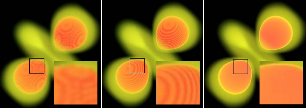
On the other side post-classification reverses the order of operations. This type of classification is characterized by the application of the transfer function after the interpolation of s(x) from the scalar values of the discrete sampling points. The results of both pre- and post-classification can be compared in Figure 1.

Figure 1: Direct volume rendering without illumination, pre-classified (left), post-classified (middle) and pre-integrated (right)

3.3 Pre-Integrated Classification

As discussed at the end of Section 3.1 to gather better visual results, the approximation of the volume rendering integral has to be improved. Röttger et al. [12] presented a pre-integrated classification method that has been adapted for hardware accelerated direct volume rendering by Engel et al. [3]. The main idea of pre-integrated classification is to split the numerical integration process. Separate integration of the continuous scalar field and the transfer functions is performed to cope with the problematic of the Nyquist frequency.
In more detail, for each linear segment one table lookup is executed, where each segment is defined by the scalar value at the start of the segment s_f, the scalar value at the end of the segment s_b and the length of the segment d. The opacity a_i of the i-th line segment is approximated by

a_i

1-exp

æ
è

ó
õ

(i+1)d

id

t(s(x(l)))dl

ö
ø

1-exp

æ
è

ó
õ

1

0

t((1-w)s_f+w s_b)d dw

ö
ø

(4)

Analogously the associated color (based on a non-associated color transfer function) is computed through

t
i

ó
õ

1

0

t((1-w)s_f+ws_b)c((1-w)s_f+ws_b)

(5)

×exp

æ
è

ó
õ

w

0

t((1-w¢)s_f+w¢ s_b)d dw¢

ö
ø

d dw.

Both functions are dependent on s_f, s_b, and d (only if lengths of the segments are not equal). Because pre-integrated classification always computes associated colors, a_iC_i in equation (2) has to be substituted by C_i.
Through this principle the sampling rate does not depend anymore on the non-linearity of transfer functions, resulting in less undersampling artifacts. Therefore, pre-integrated classification has two advantages, first it improves the accuracy of the visual results, and second fewer samples are required to achieve equal results regarding to the other presented classification methods.
The major drawback of this approach is that the lookup tables must be recomputed every time the transfer function changes. Therefore, the pre-integration step should be very fast. Engel et al. [3] proposes to assume a constant length of the segments and the usage of integral functions for t(s) and t(s)c(s) the evaluation of the integrals in equations (4) and (5) can be greatly accelerated. Adapting this idea results in the following approximation of the opacity and the associated color

a(s_f,s_b,d)

1-exp

æ
è

s_b-s_f

(T(s_b)-T(s_f))

ö
ø

(s_f,s_b,d)

s_b-s_f

(K^t(s_b)-K^t(s_f))

(6)

with the integral functions T(s)=ò₀^st(s)ds and K^t(s)=ò₀^st(s)c(s)ds. Thus, the numerical computing for producing the lookup tables can be minimized by only calculating the integral functions T(s) and K^t(s). Afterwards computing the colors and opacities according to equations (6) can be done without any further integration. This pre-calculation can be done in very short time, so providing interactivity in transfer-function changes. The quality enhancement of pre-integrated classification in comparison to pre- and post-classification can be seen in Figure 1.

3.4 Texture Based Volume Rendering

Basically there are two different approaches how hardware acceleration can be used to perform volume rendering.

3D texture-mapped volume rendering

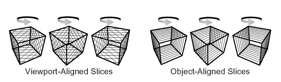
If 3D-textures are supported by the hardware (like on the ATI-Radeon family [13] or the NVIDIA GeForce 3 and 4 [15]) it is possible to download the whole volume data set as one single three-dimensional texture to hardware. Because hardware is able to perform trilinear interpolation within the volume, it is possible to render a stack of viewport-aligned polygon slices orthogonal to the current viewing direction (see Figure 2, left).
This viewport-aligned slice stack has to be recomputed every time, the viewing position changes. Finally, in the compositing step, the textured polygons are blended onto the image-plane in a back-to-front order. This is done by using the alpha-blending capability of computer graphics hardware which usually results in a semitransparent view of the volume. In order to obtain equivalent representations while changing the number of slices, opacity values have to be adapted according to the slice distance.

2D texture-mapped volume rendering

If hardware does not support 3D texturing, 2D texture mapping capabilities can be used for volume rendering. In this case, the polygon slices are set orthogonal to the principal viewing axes of the rectilinear data grid. Therefore if the the viewing direction changes by more than 90 degrees, the orientation of the slice normal has to be changed. This requires that the volume has to be represented through three stacks of slices, one for each slicing direction respectively (see Figure 2, right).
2D texturing hardware does not have the ability to perform trilinear interpolation (as performed by 3D texturing hardware), so it is substituted by bilinear interpolation within each slice, which is supported by hardware. This results in strong visual artifacts due to the fact of the missing spatial interpolation. Another major drawback of this approach in contrast to the previous one is the high memory requirements, because 3 instances of the volume data set have to be hold in memory. To obtain equivalent representations, the opacity values have to be adopted according to the slice distance between adjacent slices in direction of the viewing ray.

Figure 2: Alignment of texture slices for 3D texturing on the left, and 2D texturing on the right (image from Rezk-Salama et al. [11])

3.5 High-Quality Filtering

Commodity graphics hardware can also be exploited to achieve hardware-accelerated high-quality filtering with arbitrary filter kernels, as introduced by Hadwiger et al. [4]. In this approach filtering of input data is done by convolving it with an arbitrary filter kernel stored in multiple texture maps. As usual, the base is the evaluation of the well-known filter convolution sum

g(x)=(f*h)(x)=

ëxû+m
å
i=ëxû-m+1

f[i]h(x-i)

(7)

this equation describes a convolution of the discrete input samples f[i] with a reconstruction filer h(x) of (finite) half-width m.
To be able to exploit standard graphics hardware to perform this computation, the standard evaluation order (as used in software-based filtering) has to be reordered. Instead of gathering all input sample contributions within the kernel width neighborhood of a single input sample, this method distributes all single input sample contributions to all relevant output samples. The input sample function is stored in a single texture and the filter kernel in multiple textures. Kernel textures are scaled to cover exactly the contributing samples. The number of contributing samples is equal to the kernel width. To be able to perform the same operation for all samples at one time, the kernel has to be divided into several parts, to cover always only one input sample width. Such parts are called filter tiles.
Instead of imagining the filter kernel being centered at the "current" output sample location, an identical mapping of input samples to filter values can be achieved by replicating a single filter tile mirrored in all dimensions repeatedly over the output sample grid. The scale of this mapping is chosen, so that the size of a single tile corresponds to the width from one input sample to the next.
The calculation of the contribution of a single specific filter tile to all output samples is done in a single rendering pass. So the number of passes necessary is equal to the number of filter tiles the filter kernel used consists of. Due to the fact that only a single filter tile is needed during a single rendering pass, all tiles are stored and downloaded to the graphics hardware as separate textures. If a given hardware architecture is able to support 2n textures at the same time, the number of passes can be reduced by n.
This method can be applied for volume rendering purposes by switching between two rendering contexts. One for the filtering and one for the rendering algorithm, whereas first a textured slice is filtered according to the just described method, and afterwards the filtered output is then used in the standard volume rendering pipeline. 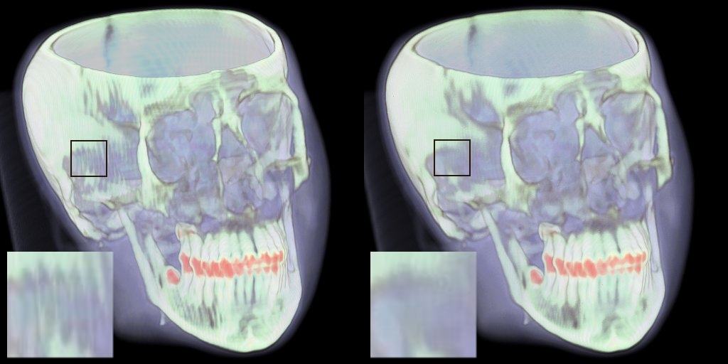This is not as easy as it sounds, thus implementation difficulties are described in more detail in section 4.1. For results see Figure 3.

Figure 3: Pre-integrated classification without pre-filtered slices (left) and applying hardware-accelerated filtering (right).

4 Implementation

Our current implementation is based on a graphical user interface programmed in java, and a rendering library written in c++. For proper usage of the c++ library in java, e.g. for parameter passing, we exploit the functionality of the java native interface, which describes how to integrate native code within programs written in java. Due to the fact that our implementation is based on the OpenGL API, we need a library that maps the whole functionality of the native OpenGL library of the underlying operating system to java. Therefore we use the GL4Java library [14]. The following detailed implementation description will only cover the structure of the c++ rendering library, because all rendering functionality is encapsulated there.
On startup of the framework, the graphics adapter currently installed in the system is detected automatically. Regarding to the OpenGL extensions that are supported by the actual hardware the rendering modes that are not possible are disabled. Through this procedure, the framework is able to support a lot of different types of graphics adapters without changing the implementation.
Anyway the framework is primarily based on graphics chips from NVidia and from ATI, because the OpenGL-extensions provided by these two vendors are very powerful features, which can be exploited very well for diverse direct volume rendering techniques. Minimum requirements for our application are multi-texturing capabilities. Full functionality includes the exploitation of the so called texture shader OpenGL extension and the register combiners provided by NVidia as well as the fragment shader extension, provided by ATI.
Basically the texture based volume rendering process can be split up into several principal subtasks. Each of these tasks is realized in one or more modules, to provide easy reuse possibilities. Therefore the implementation of new algorithms and the support of new hardware-features (OpenGL-extensions) is very simple by only extending these modules with additional functionality. The overall rendering implementation need not to be changed to achieve support of new techniques or new graphics chips.

Texture definition

As described in section 3.4, in the beginning of the rendering process the scalar volume data must be downloaded to the hardware. According to the selected rendering mode, this is either be done as one single three-dimensional texture or as three stacks of two-dimensional textures.
The selected rendering mode additionally specifies the texture format. In our context texture format means, what values are presented in a texture. Normally, RGBA (Red, green, blue and alpha component) color values are stored in a texture, but in volume rendering, other information as the volume gradient or the density value have to be accessed during the rasterization stage. 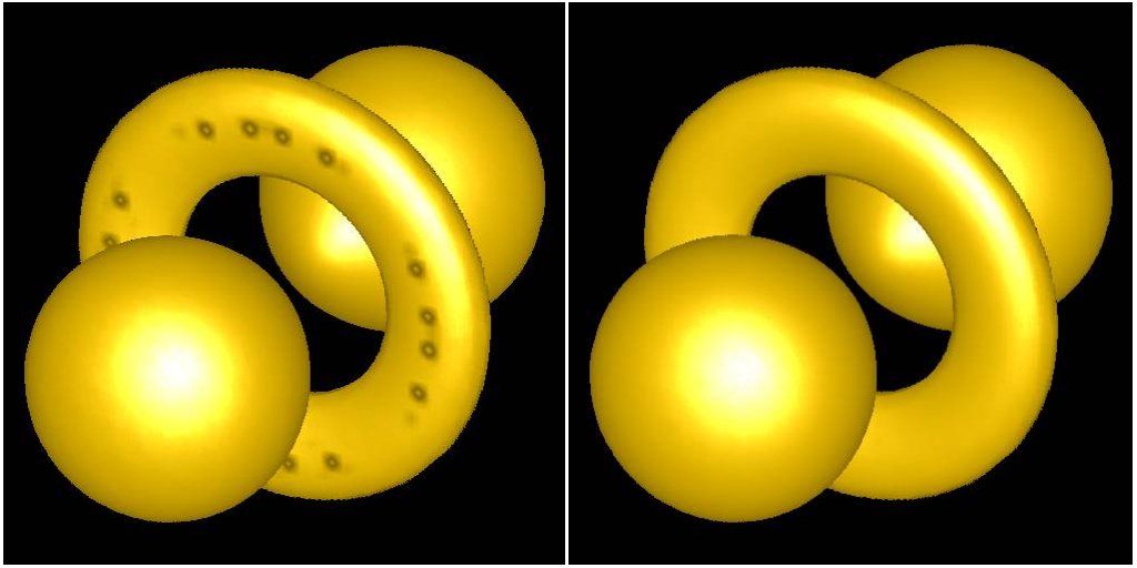For gradient vector reconstruction, we have implemented a central-difference filter and additionally a sobel-operator, which results in a great quality enhancement in contrast to the central-difference method, avoiding severe shading artifacts (see Figure 4).

Figure 4: Gradient reconstruction using a central-difference filter (left) and avoiding the shading artifacts (black holes) by using a sobel-operator (right)

When performing shading calculations, RGBA textures are usually employed, that contain the volume gradient in the RGB components and the volume scalar in the ALPHA component. As in pre-integrated rendering modes the scalar data has to be available in the first three components of the color vector, it is stored in the RED component. The first gradient component is stored in the ALPHA component in return. Another exception occurs for rendering modes, which are based on gradient-weighted opacity scaling, where the gradient magnitude is stored in the ALPHA component. Through the limitation of only four available color components, it is trivial that for the combination of some rendering modes it is not possible to store all the required values for a single slice in only one texture.

Projection

The geometry used for direct volume rendering, in contrast to other methods, e.g. iso-surface extraction, is usually very simple. Due to the fact that texture-based volume rendering algorithms usually perform slicing through a volume, the geometry only consists of one quadrilateral polygon for each slice. To obtain correct volume information for each slice, each polygon has to be bound to the corresponding textures that are required for the actual rendering mode. In addition, the texture coordinates have to be calculated accordingly. Usually this is a very simple task.
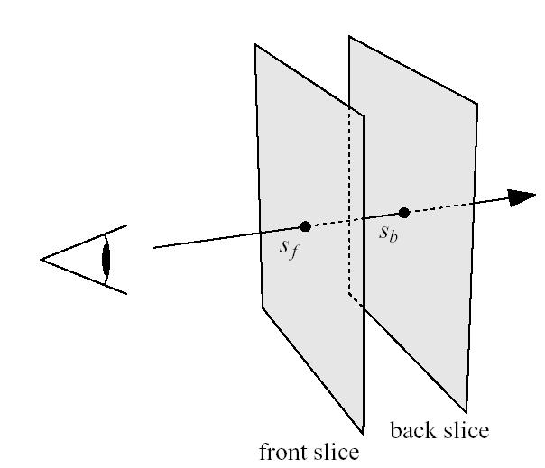
Just for 2D-texture based pre-integrated classification modes, it is a little bit more complex. Instead of the general slice-by-slice approach, this algorithm renders slab-by-slab (see Figure 5) from back to front into the frame buffer. A single polygon is rendered for each slab with the front and the back texture as texture maps. To have texels along all viewing rays projected upon each other for the texel fetch operation, the back slice must be projected onto the front slice. This projection is performed by adapting texture coordinates for the projected texture slice, which always depends on the actual viewing position.

Figure 5: A slab of the volume between two slices. The scalar values on the front and on the back slice for a particular viewing ray are called s_f and s_b (image from Engel et al. [3])

Compositing

Usually in hardware accelerated direct volume rendering approaches, the approximation of the volume rendering integral is done by back-to-front compositing of the rendered quadriliteral polygon slices. This should be performed according to equation (3). In general this is achieved by blending the slices into the frame buffer with the OpenGL blending function glBlendFunc(GL_ONE,GL_ONE_MINUS_SRC_ALPHA).
This is a correct evaluation only, if the color-values computed by the rasterization stage are associated colors. If they are not pre-multiplied (e.g. gradient-weighted opacity modes produce non-associated colors), then the blending function must be glBlendFunc(GL_SRC_ALPHA,GL_ONE_MINUS_SRC_ALPHA).
Iso-surface reconstruction in hardware is in general accomplished by cleverly exploiting the OpenGL alpha-test (e.g. glAlphaFunc(GL_GREATER, 0.4)) to display the specified isovalues only.
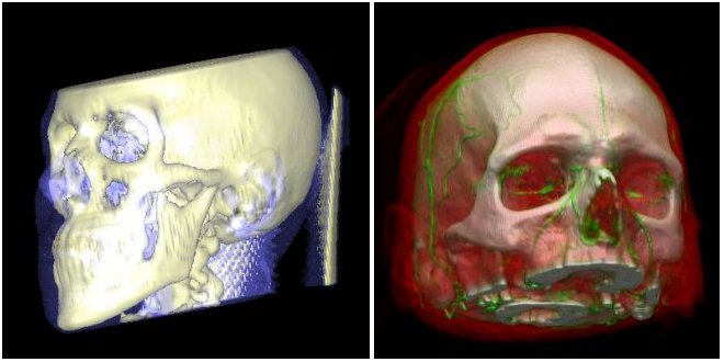
These two techniques can be combined for rendering semi-transparent iso-surfaces (see Figure 6, left), where the alpha-test is used for rejecting all fragments not belonging to an iso-surface, and afterwards the slices are blended into the frame buffer, as described above. A detailed description of iso-surface reconstruction follows in Section 4.1.

Register settings

Depending on the selected rendering mode, during the rasterization process, the actual performed rendering technique often needs more input data than available through the slice textures (in general hold gradient and/or density information). For shading calculations the direction of the light source must be known. When modelling specular reflection the rasterization stage requires not only the light direction, but also the direction to the viewer's eye, because a halfway vector is used to approximate the intensity of specular reflection. Additionally some rendering modes need to access specific constant vectors, to perform dot-products for gradient reconstruction for example. This information has to be stored at a proper place. Therefore NVidia and ATI provide some special registers which can be accessed during rasterization process when using the register combiners extension or the fragment shader extension.
The register combiners extension, as described in [11], is able to access two constant color registers (in addition to the primary and secondary color), which is not sufficient for complex rendering algorithms. In the GeForce3 graphics chip, NVidia has extended the register handling by introducing the register combiners2 extension, providing per-combiner constant color registers. This means that each combiner-stage has access to its own two constant registers, so the maximum number of additional information, provided by RGBA vectors, is the number of combiner stages multiplied by two, respectively sixteen on GeForce3. In contrast all ATI graphics chips (e.g. Radeon 8500, ...), that support the OpenGL fragment shader extension provide access to an equal number of constant registers, namely eight.
Due to the fact that miscellaneous rendering modes need different information contained in the constant registers, the process of packing the required data into the correct registers is more complex than it sounds. In addition these constant settings intensely influence the programming of the rasterization stage, where each different register setting requires a new implementation of the rasterization process.

Figure 6: Semi-transparent iso-surface rendering (left) and pre-integrated volume rendering (right) of different human head data sets.

4.1 NVIDIA vs. ATI

As mentioned above our current implementation supports several graphics chips from NVidia as well as several graphics chips from ATI. In this section we discuss the differences between realizations of several rendering algorithms according to the hardware-features supported by NVidia and ATI. The main focus is set on the programming of the flexible rasterization hardware, enabling advanced rendering techniques like per pixel-lighting or advanced texture-fetch methods. The differences will be discussed in detail by showing some implementation details for some concrete rendering modes after giving an short overview of rasterization hardware differences in OpenGL.
In general the flexible rasterization hardware consists of multi-texturing capabilities (allowing one polygon to be textured with image information obtained from multiple textures), multi-stage rasterization (allowing to explicitly control how color-, opacity- and texture-components are combined to form the resulting fragment, per-pixel shading) and dependent texture address modification (allowing to perform diverse mathematical operations on texture coordinates and to use these results for another texture lookup).

NVidia

On graphics hardware with an NVidia chip, this flexibility is provided through several OpenGL extensions, mainly GL_REGISTER_COMBINERS_NV and GL_TEXTURE_SHADER_NV. When the register combiners extension is enabled, the standard OpenGL texturing units are completely bypassed and substituted by a register-based rasterization unit. This unit consists of two (eight on GeForce3,4) general combiner stages and one final combiner stage.
Per-fragment information is stored in a set of input registers, and these can be combined, i.e. by dot product or component-wise weighted sum, the results are scaled and biased and finally written to arbitrary output registers. The output registers of the first combiner stage are then input registers for the next stage, and so on.
When the per-stage-constants extension is enabled (GL_PER_STAGE_CONSTANTS_NV), for each combiner stage two additional registers are available, that can hold arbitrary data, otherwise two additional registers are available too, but with equal contents for every stage.
The texture shader extension provides a superset of conventional OpenGL texture addressing. It provides a number of operations that can be used to compute texture coordinates per-fragment rather than using simple interpolated per-vertex coordinates. The shader operations include for example standard texture access modes, dependent texture lookup (using the result from a previous texture stage to affect the lookup of the current stages), dot product texture access (performing dot products from texture coordinates and a vector derived from a previous stage) and several special modes.
The implementation of these extensions results in a lot of code, because the stages have to be configured properly, and an assembler like programming is not provided.

ATI

On graphics hardware with an ATI Radeon chip, this flexibility is provided through one OpenGL extension, GL_FRAGMENT_SHADER_ATI. Generally this extension is very similar to the the extensions described before, but encapsulates the whole functionality in a single extension. The fragment shader extension inserts a flexible per-pixel programming model into the graphics pipeline in place of the traditional multi-texture pipeline. It provides a very general means of expressing fragment color blending and dependent texture address modification.
The programming model is a register-based model and the number of instructions, texture lookups, read/write registers and constants is queryable. E.g. on the ATI Radeon 8500 there are six texture fetch operations and eight instructions possible, both two times during one rendering pass, yielding maximum of sixteen instructions in total.
One advantageous property of the model is a unified instruction set used throughout the shader. That is, the same instructions are provided when operating on address or color data. Additionally, this unified approach simplifies programming (in contrast to the above presented NVidia extensions), because only a single instruction set has to be used and the fragment shader can be programmed comparable to an assembler language.
This tremendously reduces the amount of produced code and therefore accelerates and simplifies debugging. For these reasons and because up to six textures are supported by the multi-texturing environment, ATI graphics chips provide powerful hardware features to perform hardware-accelerated high-quality volume rendering.

Pre- and Post-classification

As described in detail in Section 3.2, pre- and post-classification differ in the order of the reconstruction step and the application of the transfer function.
Since most NVidia graphics chips support paletted textures (OpenGL extension GL_SHARED_TEXTURE_PALETTE_EXT), pre-classified volume rendering is easy to implement. Paletted textures means that instead of RGBA or luminance, the internal format of a texture is an index to a color-palette, representing the mapping of a scalar value to a color (defined by transfer-function). This lookup is performed before the texture fetch operation (before the interpolation), thus pre-classified volume rendering is performed. Since there is no similar OpenGL-extension supported by ATI graphics chips, rendering modes, based on pre-classification are not available on ATI hardware.
Post-classification is available on graphics-chips from both vendors, in case that advanced texture-fetch possibilities are available. As described in the beginning of this section when using the texture- and fragment-shader, dependent texture lookups can be performed. This feature is exploited for post-classification purposes. The transfer function is downloaded as a one-dimensional texture and for each texel, fetched by the given per-fragment texture coordinates, the scalar value is used as a lookup coordinate into the dependent 1D transfer-function texture. Thus post-classification is available, because the scalar value obtained from the first texture fetch has been bi- or trilinearly filtered, dependent on whether 2D or 3D volume-data textures are employed, and the transfer-function is applied afterwards.

Pre-integration

As post-classification, pre-integrated classification can also be performed on graphics-chips from both vendors if texture shading is available. The pre-integrated transfer-function, since dependent on two scalar values (s_f from the front and s_b from the back slice, see Figure 5 and Section 3.3 for details) is downloaded as a two-dimensional texture, containing pre-integrated color and opacity values for each of the possible combinations of front and back scalar values.
For each fragment, texels of two adjacent slices along each ray through the volume are projected onto each other. Then the two fetched texels are used as texture coordinates for a dependent texture lookup into the 2D pre-integration texture. To extract the scalar values, usually stored in the red component of the texture, the dot product with a constant vector v=(1,0,0)^T is applied. These values are then used for the lookup and the resulting fetched texel is then used for lighting calculations. 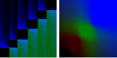An example of a pre-integration dependent texture is shown in Figure 7.

Figure 7: Dependent textures for multiple iso-surfacing (left) and pre-integrated classification (right)

Iso-surface reconstruction

The standard approach to render single iso-surfaces (as proposed by Westermann and Ertl [16]) without extracting any polygonal representation cleverly exploits the OpenGL alpha test. If the texture describing the volume contains the volume density in its alpha component, the volume is then rendered into the frame buffer using the alpha-test to compare the data value with a specified iso-value. Through this procedure a voxel is only rendered if its density value is, e.g., larger or equal to the iso-value, limiting the number of possible iso-surfaces to only one non-transparent.
Multi-stage rasterization is then exploited to perform shading with multiple light-sources as well as the addition of ambient lighting. The voxel gradient is stored in the RGB components of the texture and the available dot product is used to calculate the light intensity. The possibility of using colored light sources is also provided. If only 2D textures are available the approach of Rezk-Salama et al. [11] to produce intermediate slices on the fly can be combined with iso-surface reconstruction, resulting in better image quality. Figure 8 shows a sample register combiner setup.

Figure 8: Register combiner setup for shaded isosurfaces (image from Rezk-Salama et al. [11])

The presented usage of dependent texture lookups can also be employed to render multiple isosurfaces. The basic idea is to color each ray segment according to the first isosurface intersected by the ray segment. So the dependent texture contains color, transparency, and interpolation values (IP=(s_iso-s_f)/(s_b-s_f)) for each combination of back and front scalar. To differ between ray segments that do or do not intersect an isosurface an interpolation value of 0 is stored for ray segments not intersecting an isosurface. 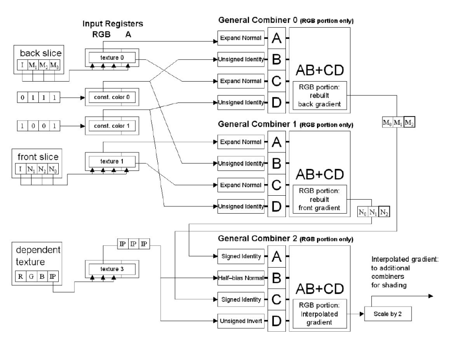The interpolation values are then stored in the alpha channel in the range 128 to 255 and the alpha-test is used again to discard voxels not belonging to an isosurface. For lighting purposes the gradient of the front and back slice has to be rebuilt in the RGB components and the two gradients have to be interpolated depending on the given isovalue. The implementation of this reconstruction using register combiners is shown in Figure 9.
The main disadvantage of this method is that the transparency, which is usually freely definable for each isosurface's back and front face, is now constant for all isosurfaces' faces. This problem can be overcome by storing the interpolation values in the blue component of the dependent texture. Now the transparency for each isosurface can be freely defined but the blue color channel has to be filled with a constant value that is equal for all isosurfaces' back and front faces. The alpha test is exploited by assigning 0.0 to the alpha channel of each texel not belonging to an isosurface. Figure 7 shows a dependent texture for multiple isosurfaces.

Figure 9: Register combiner setup for gradient reconstruction and interpolation with interpolation values stored in alpha (image from Engel et al. [3])

4.2 Problems

When applying the hardware accelerated high quality filtering method (see Section 3.5) in combination with an arbitrary rendering mode, we have to cope with different rendering contexts. One context for the rendering algorithm and one for the high quality filtering. A single slice is rendered into a buffer, this result is then used in the filtering context to apply the specified filtering method (e.g. bi-cubic), and this result is then moved back into the rendering context, to perform the compositing step. More difficult is the case of combining the filtering with preintegration, where two slices have to be switched between the rendering contexts. Through different contexts the geometry and the OpenGL state handling is varying depending on whether filtering is applied or not. It is a challenge to define and provide the correct data in the right context and not mixing up the complex state handling. Although the performance is not so high, the resulting visualizations are very convincing (see Figure 3).
Another problem that occurs when realizing such a large framework is that the performance that usually is achieved by the varying algorithms can not be guaranteed. We tested our framework on a NVIDIA Geforce3 graphics board. For direct volume rendering (all possible features enabled) of a volume with a resolution of 128³ we achieved ca 12 fps for pre-, 10 fps for post- and 6 fps for pre-integrated classification. For a volume with a resolution of 256³ we achieved ca 5 fps for pre-, 4.5 fps for post- and 4 fps for pre-integrated classification. For isosurface rendering of a volume with a resolution of 128³ we achieved ca 12 fps for the standard and 6 fps for the dependent texture approach. For a volume with a resolution of 256³ ca 4 fps for the standard and 1 fps for the dependent texture approach.
Furthermore when performing shading, rendering datasets with dimensions over 256³ results in a heavy performance loss, caused by the memory bottle neck. Which means that not the whole data set can be downloaded to the graphics adapter memory, instead of, the textures are transferred between the main and the graphics memory.

5 Conclusions and Future Work

On the basis of standard 2D- and 3D-texture based volume rendering and several high quality rendering techniques, we have presented a flexible framework, which integrates several different direct volume rendering and iso-surface reconstruction techniques that exploit rasterization hardware of PC graphics boards in order to significantly improve both performance and image quality. Additionally the framework can easily be extended with respect to support of new OpenGL extensions and implementation of new rendering algorithms, by only expanding the proper modules. The framework supports most current low-cost graphics hardware and provides comparison possibilities for several hardware-accelerated volume visualizations with regard to performance and quality.
In the future we plan the integration of non-photorealistic rendering techniques to enhance volume visualizations. To overcome the problem that different graphics chips require different implementations, we will try the usage of a high-level shading language.

6 Acknowledgements

This work was carried out as part of the basic research on visualization (http://www.VRVis.at/vis/) at the VRVis Research Center Vienna, Austria (http://www.VRVis.at/), which is funded by an Austrian governmental research project called Kplus.
Special thanks to Markus Hadwiger and Helwig Hauser for patient supervision.

References

[1]: James F. Blinn. Jim Blinn's corner: Compositing. 1. Theory. IEEE Computer Graphics and Applications, 14(5):83-87, September 1994.
[2]: Brian Cabral, Nancy Cam, and Jim Foran. Accelerated volume rendering and tomographic reconstruction using texture mapping hardware. In 1994 Symposium on Volume Visualization, pages 91-98. ACM SIGGRAPH, October 1994.
[3]: Klaus Engel, Martin Kraus, and Thomas Ertl. High-quality pre-integrated volume rendering using hardware-accelerated pixel shading. In Proceedings of the ACM SIGGRAPH/EUROGRAPHICS workshop on on Graphics hardware, pages 9-16. ACM Press, 2001.
[4]: Markus Hadwiger, Thomas Theußl, Helwig Hauser, and Eduard Gröller. Hardware-accelerated high-quality reconstruction on PC hardware. In Proceedings of the Vision Modeling and Visualization Conference 2001 (VMV-01), pages 105-112, Berlin, November 21-23 2001. Aka GmbH.
[5]: Philippe Lacroute and Marc Levoy. Fast volume rendering using a shear-warp factorization of the viewing transformation. Computer Graphics, 28(Annual Conference Series):451-458, July 1994.
[6]: Marc Levoy. Display of surfaces from volume data. IEEE Computer Graphics and Applications, 8(3):29-37, May 1988.
[7]: Marc Levoy. Efficient ray tracing of volume data. ACM Transactions on Graphics, 9(3):245-261, July 1990.
[8]: William E. Lorensen and Harvey E. Cline. Marching cubes: A high resolution 3D surface construction algorithm. Computer Graphics, 21(4):163-169, July 1987.
[9]: Nelson Max. Optical models for direct volume rendering. IEEE Transactions on Visualization and Computer Graphics, 1(2):99-108, June 1995. ISSN 1077-2626.
[10]: Michael Meißner, Ulrich Hoffmann, and Wolfgang Straßer. Enabling classification and shading for 3D texture mapping based volume rendering using openGL and extensions. In IEEE Visualization '99, pages 207-214, San Francisco, 1999. IEEE.
[11]: C. Rezk-Salama, K. Engel, M. Bauer, G. Greiner, and T. Ertl. Interactive volume rendering on standard PC graphics hardware using multi-textures and multi-stage rasterization. pages 109-118.
[12]: Stefan Röttger, Martin Kraus, and Thomas Ertl. Hardware-accelerated volume and isosurface rendering based on cell-projection. pages 109-116. IEEE Computer Society Technical Committee on Computer Graphics, 2000.
[13]: ATI web page. http://www.ati.com/.
[14]: Jausoft GL4JAVA web page. http://www.jausoft.com/gl4java.html/.
[15]: NVIDIA web page. http://www.nvidia.com/.
[16]: Rüdiger Westermann and Thomas Ertl. Efficiently using graphics hardware in volume rendering applications. In SIGGRAPH 98 Conference Proceedings, Annual Conference Series, pages 169-178. ACM SIGGRAPH, Addison Wesley, July 1998.