|
|
Brno University of Technology |
| Faculty of Information Technology | |
| Department of Computer Graphics and Multimedia |
|
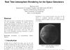
Real Time Atmosphere Rendering for the Space Simulators | |
| by Radovan Josth | ||
Abstract
This paper presents an algorithm and its implementation for the atmosphere rendering. It utilizes the Cg programming language for both the Vertex and the Pixel shader. The algorithm consists of five steps, every step generating the depth textures from the Depth buffer. The depth textures are non-power-of-two textures because we can not guarantee power-of-two screen size. The main part of the atmosphere rendering algorithm is using a programmable pixel pipeline.
1 Introduction
Looking down on Earth from space, one can see very beautiful transparent blue haze around the planet which covers the relief of the mountains and the seas. The Earth is enveloped by a vast amount of air called the atmosphere. If we fly down to this haze we can observe that the relief of the mountains and the seas is more colored and the intensity of blue transparent color slightly decreases, but the stars and the black color of the space is fading out in a glow of the shiny atmosphere. If we look on Earth from a distance, we can see a glowing tiny ring around the Earth.
White hovering objects in real atmosphere are the clouds. The clouds are very complicated objects with various densities. Density and width are very important parameters for the color of the clouds. For simplification, we do not render clouds in this work, but it can be extended to cover this issue.
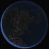
Realistic atmosphere rendering is a complex work, requiring much more computational power than for a simple atmosphere. In games or space simulators we can not use the CPU just for the atmosphere rendering, we need it also for physics or something else. The GPU is utilized to decrease the load of the CPU. For the implementation of the supporting algorithm we use the C/C++ language and for the main algorithm we use the programmable pipeline. The shaders are programmed in the Cg language developed by NVidia, both for the Vertex and the Pixel Shaders. The fixed pipeline is turned off while the atmosphere is rendered. The output of this algorithm is very accurate because every pixel on the screen is computed separately according to the atmosphere depth. Example screen shot of this algorithm is in Figure.1.
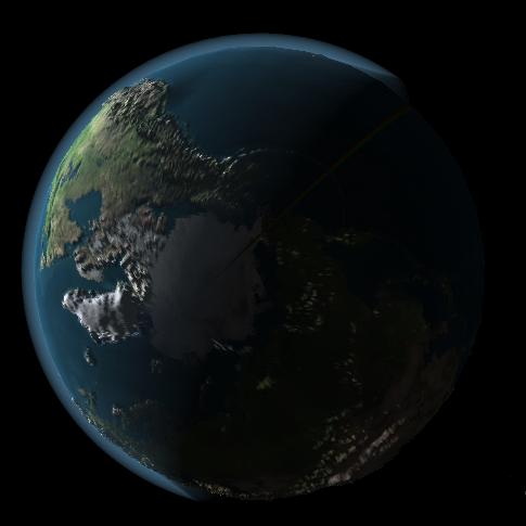
Figure 1: The atmosphere rendered by this algorithm
Similar algorithms were presented in the past. Many of these algorithms render atmosphere from the inside of it and don't consider a view from the space towards the Earth. These algorithms are mainly designated for flight simulators. Very precise rendering of the atmosphere was introduced by Ralf Stokholm Nielsen (Sept. 2003) [3]. Algorithm presented by Tomoyuki Nishita, Takao Sirai, Katsumi Tadamura and Eihachiro Nakamae [2] was mainly designated for view from the space. The atmosphere seems to be reddish when looking from the back side of it. List and descriptions of other algorithms can be found on the web [4]
2 The theoretical background
The atmosphere is relatively thin compared to the size of the earth and fades away with increasing distance from the earth's surface. The earth's atmosphere is categorized into 4 layers - troposphere, stratosphere, mesosphere and thermosphere. The troposphere where all the weather takes place and stratosphere, the two closest layers to earth's surface constitute more than 99% of the atmosphere. The troposphere and the stratosphere extend up to 12 km and 53 km respectively from the earth's surface, these two layers are almost invisible. The earth's atmosphere is composed of many gases. Gravity holds the atmosphere close to the earth's surface and explains why the density of the atmosphere decreases with altitude.
The density and the pressure of the atmosphere vary with the altitude and depend on the solar heating and the geomagnetic activity. The simplest is an exponential fall off model where the pressure and the density decrease exponentially with the altitude.
The back side of the atmosphere is slightly illuminated by the stars and in some cases by the Moon. The real atmosphere color depends on light position and also on the width of the atmosphere which the light must pass through. But in this algorithm we consider only the width of the atmosphere and the shadow of the planet and we don't consider the change of the RGB proportion.
3 The Algorithm
In this section we introduce an algorithm for shadow rendering. The algorithm does not consider the color dependence between the position of the light and the atmosphere width. The atmosphere color is evaluated only from the illuminated atmosphere width and shadowed atmosphere width.
This algorithm is divided into two parts. One part is programmed in C/C++ and running on the CPU. This part: draws the shadowing object, the planet and the atmosphere; controls programmable pipeline by setting its state to enabled or disabled and setting its parameters. The second part of the algorithm is done in the pixel shader. In this part we are getting color of every single pixel of the atmosphere.
The pixel color depends on the atmosphere width. The color is composed of three parts, the atmosphere behind the shadow, inside the shadow and last, the atmosphere in the front of the shadow. For this reason we need to divide the algorithm into more steps.
1. render the depth value for the back side of the shadow
2. render the depth value for the front side of the shadow
3. render the planet
4. render the depth value for back side of the atmosphere
5. render the front side of the atmosphere
Parts 1, 2, 3, 4 are passed without a use of the pixel shader. Parts 1, 2, 4 are required only for generating the depth texture. The third part renders planet to the depth buffer and to the color buffer. In the last part we enable the pixel shader and compare the depth textures.
Shadow object is modeled with a simple cone. The shadow cone diameter is equivalent to average diameter of the planet. The color of the atmosphere in the shadow doesn't depend on the moon phase or the stars.
1.) The first step renders the depth value for the back side of the shadow, which is used for clipping in the fifth step. (Fig.2.)
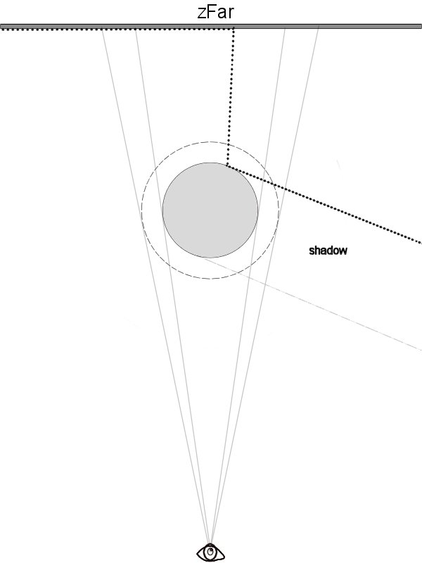
Figure 2: Back Shadow Face
2.) The second step is very similar to the first one, only one difference is between them. The second step renders the depth value for the front side of the shadow. (Fig.3.)
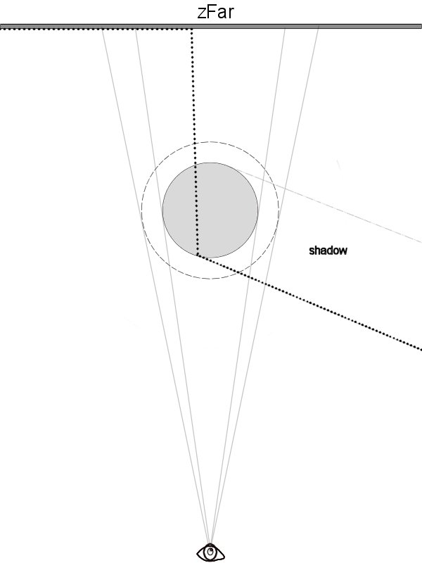
Figure 3: Front Shadow Face
Steps number one and two divide the depth values in three parts:
- the atmosphere behind the shadow
- the atmosphere inside the shadow
- the atmosphere in the front of the shadow
3.) The third step renders the planet surface into the color buffer and into the depth buffer. The depth buffer will be used later for clipping the atmosphere behind the planet. (Fig.4.)
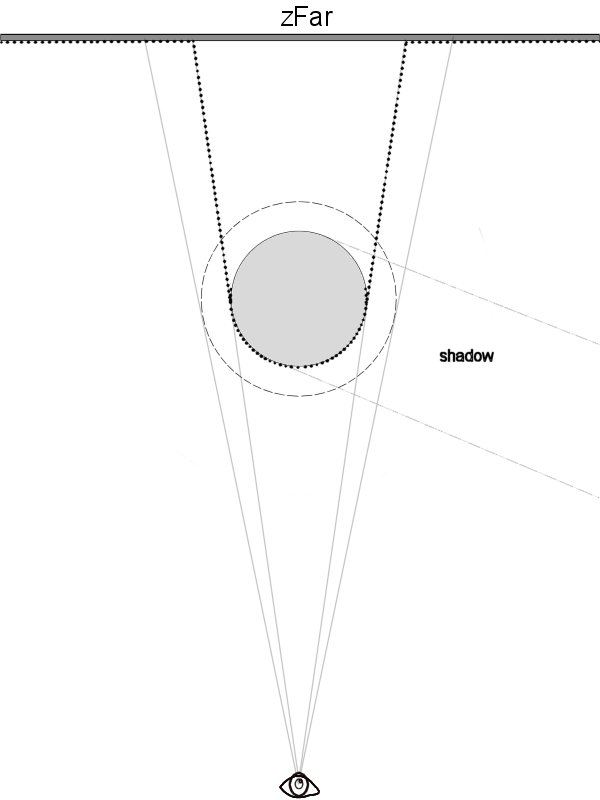
Figure 4: Planet Depth
4.) The fourth step renders the back side of the atmosphere into the depth buffer. This step divides the depth buffer into two parts: behind the atmosphere and inside or in front of the atmosphere. (Fig.5.)

Figure 5: Planet + Back Atm. Depth
Having all the depth information in the textures, we can start with creation of the atmosphere itself.
5) The main step is the fifth step. This step renders the complete atmosphere using the Pixel Shader. This step needs the four depth textures which are passed through the pixel shader parameters. Now, having these textures, we can compute the color for every pixel. Each pixel is a sum of three values:
- the atmosphere behind the shadow
- the atmosphere within the shadow
- the atmosphere in front of the shadow
These three values are computed separately. For computing the first value, the precomputed shadow depth values are required. Every value in the shadow depth buffers must be clipped with the front and the back side of the atmosphere and the planet depth textures. (Fig.6.)

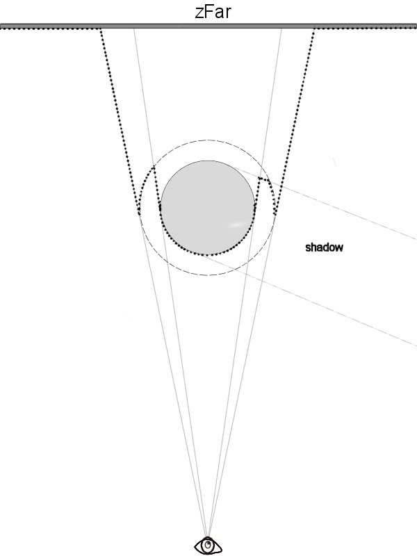
Figure 6: Front(a) and Back(b) side of clipped shadow
The atmosphere behind the Shadow
For the atmosphere color behind the shadow we use the clipped front shadow depth value (Fig.6a.) and the depth value from step 4.) (Fig.5.)

Figure 7: The atmosphere width behind the shadow
The atmosphere inside the shadow
The second step is computed from the subtraction of the two clipped shadow depth values (Fig.6a, Fig.6b). We can see the result of the subtraction in Fig.8.
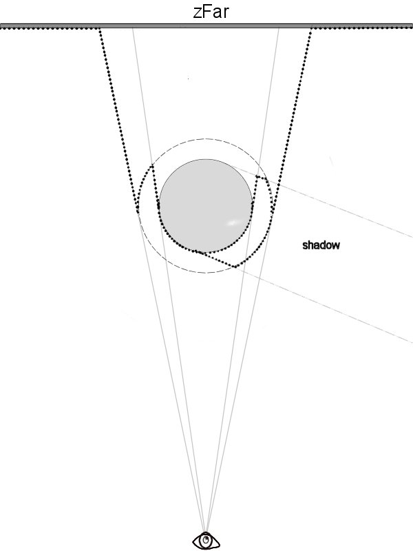
Figure 8: The atmosphere width within shadow
The atmosphere in front of the shadow
We get the third value from subtraction of the front side clipped shadow (Fig.6a) and the front side of the atmosphere.
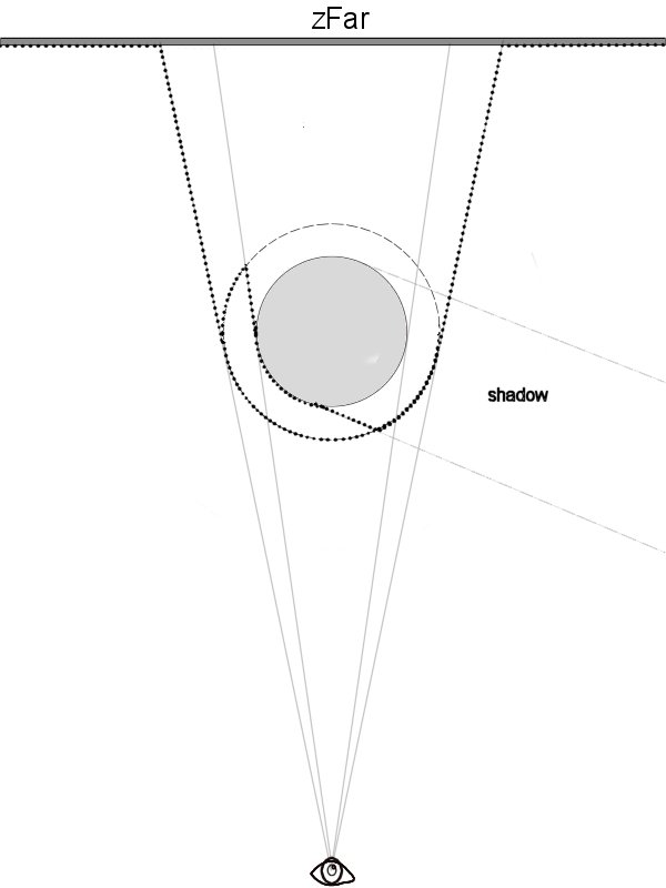
Figure 9: The atmosphere width in front of the shadow
The final illuminated atmosphere width is a sum of the first and the third value.
The second value (atm_width2) is equivalent to the width of the atmosphere in the shadow. The color of the atmosphere is now computed from atm_light and atm_width2.
4 Implementation
For implementation, the Cg language was used for pixel/vertex shaders and C/C++ for the main application program. The application is using the OpenGL standard for fast rendering. The pixel shader must be ARBFP1 or FP30.
The following problems have been faced during the experimenting with the algorithm.
- In some cases the shadow object may be closer than Z-near clipping plane, in this case an extended Pixel shader is used for changing the depth value of the fragment to z-near. This approach avoids the need of using an extra shadow cap above the atmosphere cap. Without this clipping, some errors may occur in the picture in some cases (Fig.11.).
- Next problem can be too small value of z-near clipping plane. When the observer is very close to the front side of the atmosphere, very sharp steps between separate atmosphere layers can be seen (Fig.12.). This artifact is caused by the depth buffer being non-linear and for the farthest objects (values) the depth value features too low resolution compared to the closer objects (values).
- We need non-power-of-two-textures for the depth textures. For work with these textures GL_TEXTURE_RECTANGLE_NV must be enabled and used as the target for binding textures.
Rendering of the atmosphere Step-by-step:
- Clear Buffers (Depth, Color)
- Set ColorMask to FALSE for all colors
- Render the clipped back side of the shadow
- Save the depth texture (ShadowBack)
- Render the clipped front side of the shadow
- Save the depth texture (ShadowFront)
- Clear the depth buffer
- Render the planet
- Render the back side of the atmosphere
- Save the depth texture (PlAtDepth)
- Enable the Pixel Shader
- Set parameter ZParam for the pixel shader (constants for linearization)
- Render the front side of the atmosphere
Depth Buffer Linearization:
As we know, the depth buffer is not linear. Closer objects are more detailed. When we want to get the atmosphere width, we need to compute with the linear values. We must linearize the depth values.
z_linear = b / (z_buffer_value - a)
Where:
a = zFar / ( zFar - zNear )
b = zFar * zNear / ( zNear - zFar )
Pixel Shader code:
atmosphere.cg
5 Results
The algorithm described in this paper has been implemented and experimented with in the Microsoft Windows operating system.
All tests were performed on Athlon 3400+ with the NVidia FX5200 graphics card. Average frame rate was 9 fps at resolution 1280x1024. FX 5200 graphics card is too slow for rendering full screen picture with the Pixel Shader. Without the atmosphere rendering, we can get 26 fps. Rendered planet has got 196000 triangles. Earth sphere is very densely tessellated sphere. Mountain scale depends on the camera distance. The scale factor is changing dynamically in the programmable vertex shader. The mountain scaling is very good visual improvement because the observer will get nice look from the space down to the earth. This technique is very time-consuming and many algorithms do not use it.
6 Conclusions and Future work
The presented algorithm can be used for rendering positional fog with shadow or for nebulas. This method is very fine for the atmosphere width in rugged relief, most of other atmospheric algorithms do not consider the planet relief from the space when the relief is scaled.
Further work now continues on the atmosphere rendering from earth's surface and in the future I want to implement static/dynamic clouds which will greatly improve the visual quality of the atmosphere from the space and from the earth. Another future improvement will be rendering the eclipses. If some planet is eclipsed, the atmosphere of it must be shadowed too. This improvement will involve rendering and combining two shadowing objects.
References
[1] NVidia, Cg-Toolkit (Release 1.2, 2004)
[2] Tomoyuki Nishita, Takao Sirai, Katsumi Tadamura, Eihachiro Nakamae. Display of the Earth Taking into Account Atmospheric Scattering, SIGGRAPH, 1993
[3] Ralf Stokholm Nielsen. Real Time Rendering of Atmospheric Scattering Effects for Flight Simulators, Sept. 2003
[4] http://www.vterrain.org/Atmosphere/
Sample screenshots
| Side view | 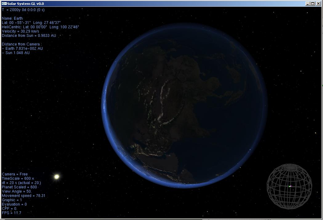 |
|
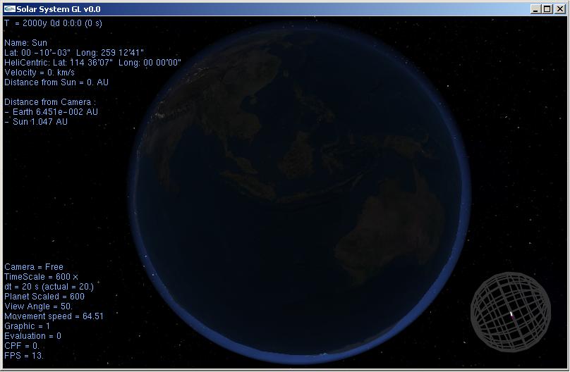
| Front side view |  |
|
|
Back side view (inside shaodwing object) |
 |
|
| Detailed view of the atmosphere width on rugged relief | 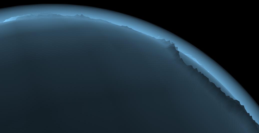 |
|
| View of the shadowing object in the scaled atmosphere | 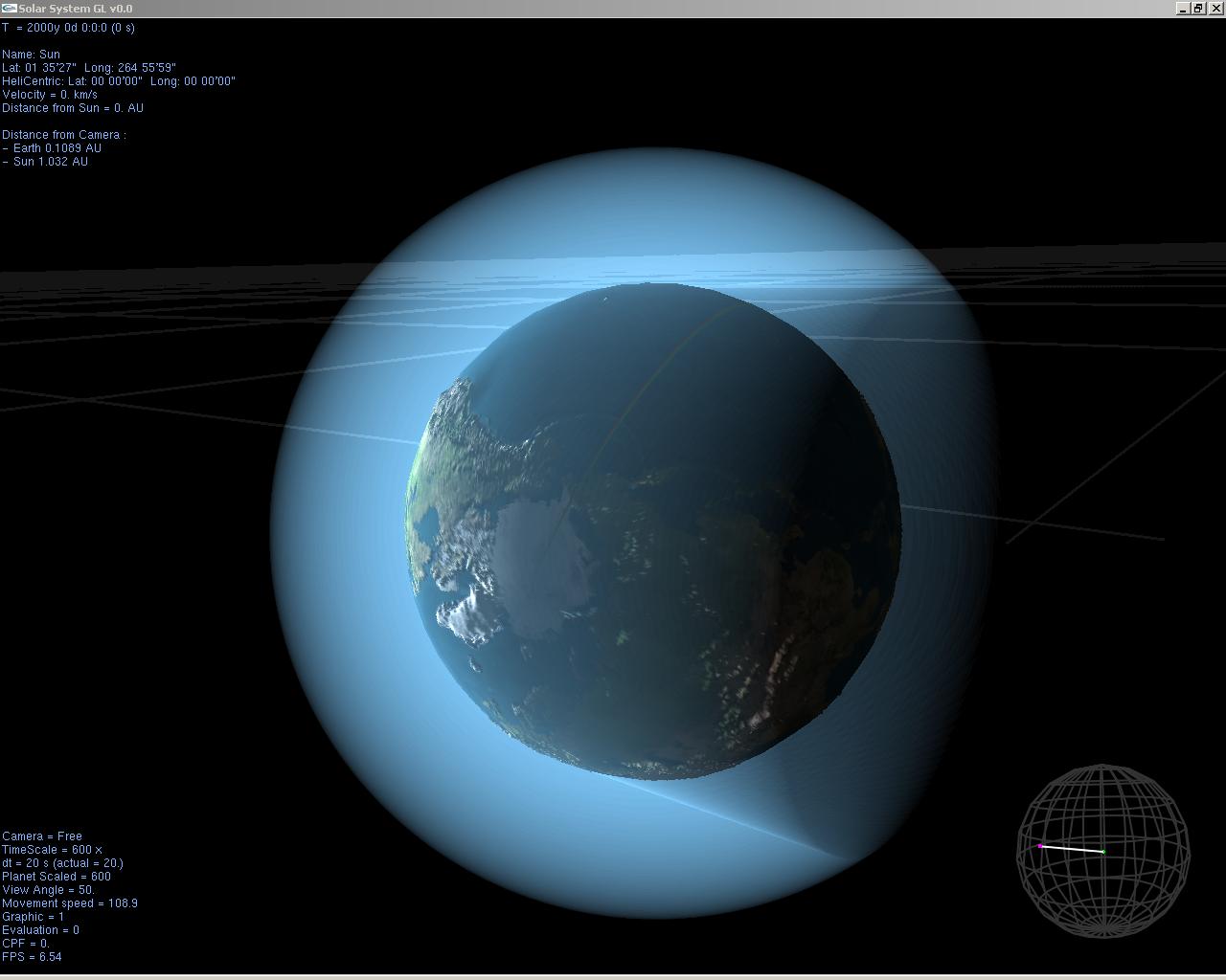 |
Download full paper
 CESCG2005-Josth Radovan.pdf (~804KB)