Accessibility Shading
The method of accessibility shading can be used to render dust covered or
tarnished surfaces that have been cleaned by a rack, that is unable to reach into
sharply concave corners and creases. These non-accessible areas tend to retain dirt or
tarnish. To treat these effects convincingly, Miller formulates several methods for
computing the accessibility of a surface.
Researchers in molecular modeling have long been concerned with defining surface
accessibility, since many chemical reactions depend on the access of one molecule to the
surface of another. The problem was first addressed quite early in 1971. This first
approach dealt with solvent molecules. The accessible surface was found by offsetting the molecule
outward by the probe radius and then offsetting inward by the same amount. In concave regions this offset
surface will be self intersecting. By trimming away these self intersecting regions, the true offset envelope
will be found. In the special
case of a solvent molecule, the fillet will be a portion of a torus (See Image 4).
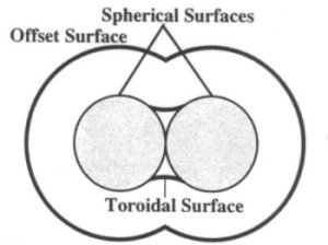
Image 4. The solvent accessible surface for a pair of spheres.
Tangent Sphere Accessibility
This first approach can be extended to a method called tangent sphere accessibility.
Surface accessibility is defined to be the radius of a sphere which may touch the surface
tangentially and not intersect any other surfaces. The size of such a sphere will depend
on the surface curvature (See Image 5) and the proximity of other surfaces (See Image 6).
Where to surfaces intersect the radius will go to zero.
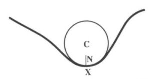
Image 5. A sphere touching a surface tangetially with the maximum allowed radius.
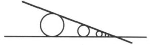
Image 6. Accessibility for two intersecting planes.
Another extension to the algorithm can be made easily to treat the presence of other
geometry, such as spheres, cylinders, and polygons correctly.
As the number of objects increases, the cost of computing the tangent-sphere accessibility increases, too (what a surprise).
For the naive
algorithm the cost is linear to the number of objects and proportional to the number of
visible pixels. One simple optimization can be reached by benefiting from pixel-to-pixel
coherence. Just like using scan line coherence, previous pixels are used to accelerate
the computation for the current pixel. The speed up can be enormous when the coherence
carries between different primitives if they are close enough together and have a similar
enough normal vector. In detail this optimization is achieved by slightly enlarging the
bound for one of the spheres. After doing that, this sphere will contain the sphere for
the adjacent pixel. This coherence may be used by always employing an enlarged or so
called ‘sloppy’ bound to find the list of overlapping objects. For the next pixel, the
new sphere is tested against the old sloppy bound. If the new sphere fits entirely within
the old bound, then the old list of overlapping surfaces may be used for this pixel. This
process continues until a sphere occurs which does not fit within the sloppy bound. In
that case a new sloppy bound has to be created and the adjacent pixels are tested against
this new sphere.
The described sloppy bound is given by expanding the exact bound by a slop margin. The
size of this slop margin is quite important. If the margin is too large, then many
surfaces will be classified as overlapping that actually do not overlap the original
bound. If the margin is too small the overlapping surfaces will have to be recomputed
from scratch for a high portion of adjacent pixels. The optimal margin will depend on the
resolution of the image.
Unfortunately, tangent sphere accessibility has a few disadvantages.
Concave creases between adjacent polygons in a mesh will always have an inaccessible
region. As the polygons become more parallel, the inaccessible region shrinks in size but
never disappears.
Offset Distance Accessibility
An alternative definition for accessibility is to consider it equal to the distance to
the nearest point on an offset of the surface, minus the offset radius. This definition is
analogous to using a spherical clearing device with an outer layer of abrasive bristles
(See Image 7).
In convex regions with no intersections, the distance is equal to the offset radius.
In concave regions this value will increase. This method can be used to compute the
accessibility of a height field algorithmically. If a height field is represented by
samples in a rectangular buffer A, then an offset of the surface may be computed in a
second buffer B as follows.
- Buffer B is initialized to have the minimum value of buffer A at every sample.
- For each sample point in buffer A, a sphere centered at the pixel’s depth and location is
scan converted into buffer B taking the maximum of the existing
value and the value for the sphere (See Image 8).
- A third buffer C is initialized to have the maximum value of the buffer B at every sample.
- For each sample point in buffer B, a sphere centered at the pixel’s depth and
location is scan converted into buffer C taking the minimum of the existing value and the
value of the sphere.
- The distance to the nearest point on the offset-offset surface may then be
approximated by taking the difference between buffer C and the original height field in buffer A.
By changing the offset radius the accessibility of different regions can be varied.
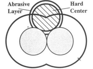
Image 7. Spherical cleaning probe with abrasive layer.
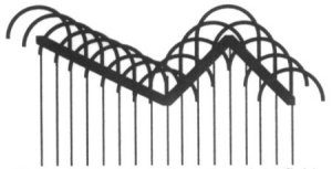
Image 8. Positive offset of a height field.
This algorithm can be adapted to work on volumetric representations as well.
In that case the model is considered to be contained within a three dimensional
rectangular array of samples in a voxel buffer A.
To offset the volume in buffer A the following steps are taken.
- A second voxel buffer B, is first initialized to be a copy of buffer A
- Then, for every voxel in buffer A which is populated and has a zero neighbor a
sphere is scan converted into voxel buffer B. The scan conversion populates voxels which lie along the span.
- Voxel buffer B then represents the offset volume.
To render the original surface with accessibility shading, the surface is scan converted
into a Z-buffer. For each surface point visible in the screen image, a corresponding point
is found in the offset voxel buffer. This buffer is the searched in an expanding sphere
until a zero valued pixel is encountered. The distance between this zero value pixel and
the original surface point is then used as the accessibility.
As conclusion some images created using tangent-sphere accessibility are shown to
demonstrate the enormous gain in realism.
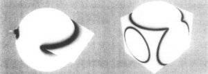
Image 9. Tangent sphere accessibility.
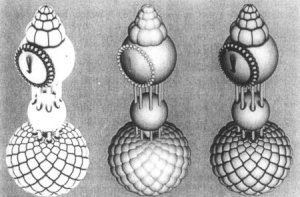
Image 10. Tangent sphere accessibility.
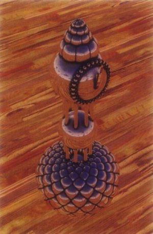
Image 11. Tangent sphere accessibility with environmental mapping.
Continue with Modeling of Metallic Patinas.