Polar Forms and Geometric Continuity of Surfaces Jana Pilnikova, Jaroslav Placek, Juraj Sofranko 3pilnikova@st.fmph.uniba.sk, Jaroslav.Placek@st.fmph.uniba.sk, Juraj.Sofranko@st.fmph.uniba.sk Faculty of Mathematic and Physics University of Comenius Bratislava, Slovakia

The paper is concerned about the question of smooth glueing of triangular Bézier patches. In the beginning polar forms are briefly explained. After that they are applied on parametric continuity. We'll obtain a geometric interpretation of C¹ and C² smoothly joined Bezier patches.

1. General Definitions

1. Bezier patches

Let points t₀,t₁,t₂ Î E² are non-colinear. Then for each u Î E² there exist unique triplet of numbers l₀(u), l₁(u), l₂(u) Î R satisfying

u = l₀(u) t₀+ l₁(u) t₁+ l₂(u) t₂; l₀(u) + l₁(u) + l₂(u) = 1.

The numbers l₀(u), l₁(u), l₂(u) are called barycentric coordinates of the point u with respect to triangle t₀,t₁,t₂.

In the next let's suppose that the points t₀,t₁,t₂ are fixly given.

Polynomial BD _ijk : E² ® R defined



is called Bernstein polynomial. Notice, that all Bernstein polynomials of degree of n (i.e. i+j+k = n) create the basis of the space of polynomials of degree at most n.

Let B: E² ® R is defined:



The restriction of this map to D t₀,t₁,t₂ is called triangular Bezier patch of degree n. Points b_ijk are control points and create a control net.

 

2. Polar forms

A map f: M ® N is linear iff it preserves the linear combination of vectors, i.e.

f(S a _iu_i) = S a _i f(u_i); u_{i Î} M, a _i Î R

f: M ® N is affine iff it preserves the affine combination of points:

f(S a _iu_i) = S a _i f(u_i); u_{i Î} M, S a _i = 1, a _i Î R

f: (M) ^{n ®} N is multilinear (multiaffine) iff it is linear (affine) in each of its arguments when the others are fixed.

f: (M) ^{n ®} N is symmetric iff its value does not depend on the order of arguments. It means

f (up _1, up _{2, . . .} up _n) = f (u_1, u_{2, . . .} u_n)

where (p ₁, p ₂, . . . p _n) is a permutation of the set (1,2, . . . n).

Now we can approach a definition of polar forms.

Let F is polynomial E^{2 ®} E^d of degree n. Then there exists unique map f: (E²) ^{n ®} E^d which is multiaffine, symmetric and has a property of diagonal, i.e. f (u_{, . . .} u) = F(u). This map is called (affine) blossom (polar form) of F.

For our cogitations linear blossoms are more useful. For this purpose we must present this two special insertions E² to E³.

u = (u_1, u₂) Þ uÙ =(u_1, u_2, 0)

u = (u_1, u₂) Þ u^- =(u_1, u_2, 1)

Linear blossom ( polar form) of the polynomial F: E^{2 ®} E³ is a map f_*: (E³)ⁿ ® E^d which is multilinear, symmetric and has a property of diagonal, i.e. f_*(u^-_{, . . .} u^-) = F(u). Such map always exists and is unique.

Linear and affine blossoms of the same polynomial F satisfy

f_* (u^-_1, u^-_{2, . . .} u^-_n) = f (u_1, u_{2, . . .} u_n); u_{i Î} E²

2. Parametric continuity

Maps F,G : E² ® E^d are parametric continuous of the order q in u _Î E² if their directional derivatives in u up to order q are the same.

The theory of polar forms can be applied on parametric continuity of surfaces. But first let's mention their two important properties:

Let F be a Bézier patch of degree n with control points b_ijk for i + j + k = n with respect to D t₀,t₁,t₂ and let f be its polar form. Then

b_ijk = f (tⁱ₀,t^j₁,t^k₂); i + j + k = n

Furtehmore if we denote Dx _{1x 2... x k} F(u) q-th directional derivative of F in u with respect to vectors x ₁, x _{2 . . . x q} then the linear blossom of F: E^{2 ®} E^d satisfy relation

(1)

where f_* is the linear blossom of F. Proofs of these properties you can find for example in [3].

We started to use a simpler an lucider multiplicative notation:

Instead of f (u_1, u_{2, . . .} u_n) we are going to write f (u₁ u_{2 . . .} u_n). By the entry f (u^n-k u₁ u_{2 . . .} u_n) we want to say that argument u occurs (n - k) times there.

Therefore, if we want to find out a vallue of a derivative of a polynomial we don't need to derive but it is enough to look at a certain value of its blossom.

From the previous theorem we get conditions for parametric continuity of two patches.

Let F,G : E^{2 ®} E^d are triangular Bezier patches and let u be a point from E². Then according to (1) F and G are continuous in u of order q iff

f_* (u^{- n-ix} _{1 . . . x i}) = g_* (u^{- n-i x} _{1 . . . x i}); i = 0, ... q

3. Geometric interpretation

 



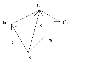
Figure 1: Mapped space

Let's denote barycentric coordinates of t^~₀ with respect to D t₀,t₁,t₂ as l₀, l₁, l₂ :

t^~_{0 =} l₀ t_{0 +} l₁ t_{1 +} l₂ t_2, l₀ > 0. Let Bézier patches F,G map this point configuration in this way:

F : D t₀,t₁,t₂ ^® E²

G : D t^~₀,t₁,t₂ ^® E²

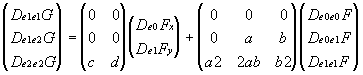
Further let b_ijk are control points of the patch F and b^~_ijk are control points of the patch G. Let's investigate a continuity of these two patches along the common edge t₁t₂. If we suppose C^o continuity, it is obvious, that derivatives in u _Î t₁t₂ with respect to e₁ are the same - it is the same Bezier curve. So that it is enough to find only one more direction which is lineary independent with e₁ with respect to which the maps F,G poses the same derivative. Then the C¹ continuity is satisfied because of the fact that Dx F(u) is linear in x for a fixed u and so the other directional derivatives can be composed from the mentioned two.

We can write:

t^~₀ - t₁ = l₀ (t₀ - t₁) + l₂ (t₂ - t₁)

e₂ = l₀ e₀ + l₂ e₁

D_e2F(u) = l₀D_e0F(u) + l₂D_e1F(u)

D_e2G(u) = D_e2F(u)

D_e2G(u) = l₀D_e0F(u) + l₂D_e1F(u)

g_*(u^{- n-1}e_2Ù ) = l₀ f_*(u^{- n-1}e_0Ù ) + l₂ f_*(u^{- n-1}e_1Ù )

. . . . .

g(t^~₀,t₁ⁱ,t₂^j) = l₀ f (t₀,t₁ⁱ,t₂^j) + l₁ f (t₁ⁱ⁺¹,t₂^j) + l₂ f (t₁ⁱ,t₂^j+1)

b^~_ijk = l₀ b_{1 i j} + l₁ b_{0 i+1 j} + l₂ b_{0 i j+1} ; i + j = n, u Î t₁t₂

And thanks to the blossoming we have simply obtained well-known geometric interpretation of the C¹ continuity:

Bézier patches F : D t₀,t₁,t₂ ^® E², G : D t^~₀,t₁,t₂ ^® E² are C¹ smoothly joined along the common boundary iff the control points b_1ij, b_{0 i+1 j}, b_1ij, b_{0 i j+1} lay in the same plane and create an affine image of the quadrangle t₀t₁t^~₀t₂.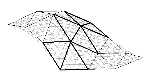



Figure 2: Geometric interpretation of C¹ continuity

After similar cogitations we can obtain not so known geometric interpretation of C² continuity:

Bézier patches F : D t₀,t₁,t₂ ^® E², G : D t^~₀,t₁,t₂ ^® E² are C² smoothly joined along the common boundary iff moreover there exist points d_i; i=1, .... n-1 such that vertexes b_2ij, b_{1 i+1 j}, d_i, b_{1 i j+1} lay in the same plane and create an affine image of the quadrangle t₀t₁t^~₀t₂ and also points d_i, b_{1 i+1 j}, b_2jk, b_{1 i j+1} are coplanar and create an affine image of the quadrangle t₀t₁t^~₀t₂ too.

 



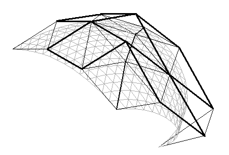
Figure 3: Geometric interpretation of C² continuity

 

4. Geometric continuity

Let F, G : E^2® E^d are maps. Let u Î E². Then F, G are in u geometric continuous of order q iff there exists such parametrication of surfaces F, G that they are parametric continuous of order q. It means:

F = F(x,y) i.e. is a function of parameters x, y

G = G(s,t)

Let's try to reparametrize the map F and express it by s, t. So x and y will be written as functions: x= x(s,t), y = y(s,t). Let both maps are now expressed in the way that they are parametric continuous in u = (s₀, t₀):

Continuity of the first degree:

F_s(u) = G_s(u) Ù F_t(u) = G_t(u)

For continuity of the second degree moreover

F_ss(u) = G_ss(u) Ù F_st(u) = G_st(u) Ù F_tt(u) = G_tt(u)

But F has to be derivated as a compound function. Let's denote

, , u Î E²

Then the relation between derivatives of F and G with respect to the original parameters can be expressed by connection matrices

(2)

(3)

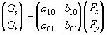
Let G' is the matrix of first derivatives of G, G'' is the matrix of its second darivatives an so on. Similary let F' is the matrix of first derrivatives of F, F'' is the matrix of its second derivatives and so on. Then the relations (2), (3) and other can be written in a simpler way:

G' = W ₁₁ F '

G'' = W ₁₂ F ' + W ₂₂ F '' (4)

G''' = W ₁₃ F ' + W ₂₃ F '' + W ₃₃ F '''

Surfaces F and G are in u geometric continuous of degree q iff there exist matrices

W _ij ; j = 1 . . . q, i = 1 . . . j

satisfying the mentioned relations.

We observe that the relations for the geometric continuity of surfaces are very similar to the ones for the geometric continuity of curves. But as a shape parameters there are matrixes W _ij instead of real numbers.

5. Geometric Continuity of Bezier Patches

Now we are going to apply the results of the previous section on the Bézier patches. Let Bézier patches F, G are defined on the quadrangle t₀t₁t^~₀t₂ like this:

F : D t₀,t₁,t₂ ^® E²

G : D t^~₀,t₁,t₂ ^® E²

Let F and G are regularly parametrized in this way:

F = F(r,s)

G = G(s,t)

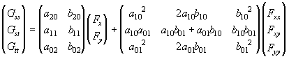
where parameter r raises in the direction e₀, s raises in the direction e₁ and t in the direction e₂ (look fig.1). We suppose C^o continuity F(0,b ) = G(b ,0). In the beginning we require geometric continuity of the first order of the patches F and G along the common boundary t₁t₂. It means that for all u from this edge there exist a matrix W ₁₁ satisfying (2). In this special case it can be written:



where a_ij, b_ij are functions of the point u.

Thanks to the fact that parameter s is common for both F and G it holds D_e1G(u) = D_e1F(u) for all u Î t₁t₂ and so a₁₀ = 0 and b₁₀ = 1 constantly.

Let a = a₀₁ b = b ₁₀ for simplicity. Then:



The result can be geometricaly interpreted: Bezier patches are in u geometric continuous of the first degree iff they have in u the same tangent plane.

Let's continue by investigating the geometric continuity of the second degree of two Bezier patches. Besides the matrix W ₁₁ with the specified form the matrices W ₁₂ and W ₂₂ must exist such that

G'' = W ₁₂ F ' + W ₂₂ F ''

If we look at (3), we can notice that all the elements of the matrix W ₂₂ are already known because it is composed only from coeficients occured in W ₁₁.

And as for W ₁₂, it's possible to proceed like in the case of W ₁₁. Because the same parameter and the derivative of the same curve is considere, it holds

D_e1e1G(u) = D_e1e1F(u) Þ a₂₀ = b₂₀ = 0

It will be a bit more complicated for the combined derivatives:

D_e1e2G(u) = D_e1(D_e2G(u))

= D_e1(aD_e0F(u) + bD_e1F(u))

= aD_e1(D_e0F(u)) + bD_e1(D_e1F(u))

= aD_e0e1F(u) + bD_e1e1F(u)

and after comparing with (3) we obtain a₁₁ = b₁₁ = 0 constantly fo all u Î t₁t₂.

The result of this observations is the next equation:



We could continue similary. After the small cogitatation above the equation for the q-th derivative

G^(q) = W _1q F ' + W _2q F '' + . . . + W _qq F ^(q) (5)

we realize that if the previous derivatives has been invastigated, new coeficients appear only in matrix asdfasdf - the q-th derivatives of the reparametrization functions are only there. Let's look at it more closely.

Let the reparametrization functions x and y are polynomials of degree m (look[2]):



From the matrix W ₁₂ it follows x_uv = a₁₁ = 0 and also y_uv = b₁₁ = 0. It means that nor x(u,v) neither y(u,v) contains combines member. Furthermore from W ₁₁ it is x_u = a₁₀ = 0, i.e. x doesn't depend on parameter u. In the case of y it is a bit different: y_u = b₁₀ = 1 constantly along the whole boundary t₁t₂. It means that y(u,v) contains u only as a linear member with coeficient ₁. The result can be written:



 

And then we obtain more specific form of W _1j: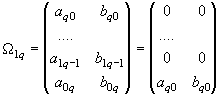



 

6. Conclusion

Let's look at the result. It seems that if the conditions of GC^q-1 smooth joining of the patches F and G has been formulated and we want to reach smoothness of q-th order, it can be determined by only two shape parameters in the matrix asdasd. There's no possibility to manipulate with other matrixes occured in the relation between G(q) and F(q) (look(5)). So the geometric continuity of curves and surfaces are very similar not only because of the form of the equation system(4) but also because of the constraints for the work with shape parameters.

7. References