Using blending functions to construct a spline curve

In this section we will construct spline curve using blending functions. We are given m+3 control points $W_{-1},\ldots,W_{m+2}$. Spline curve L(u) is defined:

$$L(u)=\sum_{i=0}^{m+1}W_{i}L^{m}_{i}(u), u\in [1,2m-1]$$ (8)

Curve L(u) interpolates control points $W_{1},\ldots,W_{m}$ because of conditions (5). Now we can count the B₂-spline control points of the curve L(u). Let us denote joining points of the curve $R_{1},\ldots,R_{m}$ and odd control vertexes $C_{0}, C_{2},\ldots,C_{2m}$. It is obvious that joining points are identical with control points interpolated by the curve: $R_{i}=W_{i},\ i=1,\ldots,m$. It is not difficult to count the odd control points: $C_{2i}=-pW_{i-1}+(p+\frac{1}{2})W_{i}+(p+\frac{1}{2})W_{i+1} -pW_{i+2}, \ i=0,\ldots,m$. 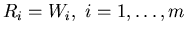In simillar way we can get also approximating spline curve. We just need to replace condition R_i=W_i by new one

R_i=aW_i-1+(1-2a)W_i+aW_i+1

where a is real parameter. This will cause new values of joining points of blending functions: Pⁱ_i-1=a, Pⁱ_i=1-2a, Pⁱ_i+1=a. For a=0 we have got the original blending functions. For $a=\frac{1}{6}$ and p=0 we will get classical B-spline curve. Implementation of spline curve is a good way to find out the best value of parameter p. For interpolating curve it seems to be $p=\frac{1}{6}$ and for $a=\frac{1}{6}$ we will simply choose B-spline value p=0. For other values of parameter a we can use linear interpolation of this two values of p. We will get: $p=\frac{1}{6}-a$.