Related Work

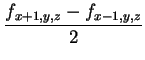
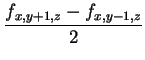
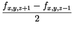
The most widely used method for gradient estimation is still the central difference operator which simply computes an averaged difference of values along each axes:

$$\frac{f_{x+1,y,z}-f_{x-1,y,z}}{2}$$ g_x =

$$\frac{f_{x,y+1,z}-f_{x,y-1,z}}{2}$$ g_y = (4)

$$\frac{f_{x,y,z+1}-f_{x,y,z-1}}{2}$$ g_z =

The same result is obtained by convolving the data set with the series $\left[\frac{1}{2},0,-\frac{1}{2}\right]$ in each dimension, the frequency response of this series can be computed analytically [4]. However, this only estimates gradients on sample positions, in between some kind of interpolation has to be performed. The frequency response of the central difference operator combined with linear interpolation (as done by Bentum et al [1]) is depicted in Fig. 1 on the right. It reveals the drawback of this method, which is that high frequencies in the data are attenuated and therefore a rather great amount of smoothing is introduced.

Bentum et al. [1] therefore proposed to use derivatives of cubic splines (which already were quite popular for function reconstruction [10]) as derivative reconstruction filters and Möller et al. [11,13,14] provide an analysis and analytic comparison of their performances. Machiraju and Yagel [8] discuss different gradient estimation schemes such as first reconstructing the function and then differentiating it or first differentiating the filter and convolving the data with that filter. An elaborated comparison is again given by Möller et al. [12].

Windowing itself is not that popular in computer graphics. Turkowski [19] used a Lanczos windowed sinc-function for decimation and interpolation of 2D image data. Goss [4] eventually proposed to use a Kaiser windowed cosc function for gradient estimation. This method will be more closely examined in Section 3.9.