ALVIS – Meeting the tremendous requirements arising with the visualization of aluminum foam samples investigated by high resolution industrial CT – modalities.

André Neubauer

e9625734@stud3.tuwien.ac.at

Armin Kanitsar

e9625009@stud3.tuwien.ac.at

Institute of Computer Graphics
Vienna University of Technology

Karlsplatz 13 / 186 / 2
Vienna / Austria

Abstract

In the last years computer tomography has been found out to be an appropriate method for non-destructive investigation of metal foam samples. Due to the small internal features of these samples high scanning resolution is needed. This results in huge data sets which cause increased computational demands in visualization.

This paper deals with methods to satisfy these demands. We will describe special algorithms like strips generation, segmentation and decimation algorithms. Furthermore we will show that some of these algorithms cooperating yield adequate visualization performance.

Keywords: Marching Cubes, segmentation, metal foam, non-destructive examination.

1. Introduction

In recent years ongoing research in material science yielded the development of high quality metal foams. Metal foams are lightweight and rigid. Furthermore metal foams feature good pressure absorbing properties. For these reasons automotive industry is a possible area of application. Also a crash energy absorbing crumple zone can be improved using metal foams. A substantial loss of weight can be reached as well as an improved deformation behavior in crash situations.

Different types of metal foams have been developed. This paper deals with metal foams featuring closed cells. There are several ways to produce metal foams. One is to add a propellant to the liquid metal at high temperatures. After cooling down small gas pockets remain. We call these holes cells. No matter what production technique is applied, it is desirable to produce cells featuring the following properties:

I. similar size

II. regular distance to each other

III. a shape similar to a sphere.

Only a sufficiently evolved combination of these properties yields high quality metal foams.

It is of special interest to material scientists to examine the interior of a sample without destroying it. We call this way of investigating samples non-destructive examination. One way to do this is to scan the sample with an industrial CT (computer tomograph) scanner and to visualize the acquired data set with the help of a special software tool. These CT modalities utilize high scanning resolution and therefore produce huge data sets.

2. Requirements

In the ALVIS project a number of requirements had to be dealt with, which are described below.

A tool had to be implemented, which should provide the possibility to visualize and analyze a CT data set in a way, that information could be gathered about the shape of the sampled object as well as its interior.

The basic requirements are listed as:

- Visualization: The most important demand was to provide means to visualize the sampled object using a computer system. Small features of the data set should not be omitted.

- Handling of big amounts of data: The investigated data sets featured sizes of several hundred MB. Therefore suitable data structures had to be used to guarantee an efficient mesh construction process.

- Interactivity: Moving around within the data set should be possible with interactive frame rates.

This includes the need for a fast visualization algorithm. There are basically two types of visualization algorithms, direct volume rendering and surface fitting algorithms. Surface fitting algorithms use an intermediate representation of the data set: the data set is reconstructed as a polygon mesh. As such a mesh can be rendered very quickly, utilizing hardware acceleration, independent of the viewpoint and the view direction those algorithms assist in satisfying the interactivity demand. The probably most prominent of the surface fitting algorithms, the Marching Cubes algorithm was chosen to be used [1].

- Segmentation: It was an important demand to supply the possibility of segmentation, which means isolating each object in the data set from its environment and associating it with a set of vertices. In the case of metal- foam visualization an object is a cell, therefore consisting of air and bounded by thin walls of metal.

- Selection: A tool should be provided to select a subset of the generated objects. The objects belonging to this subset should be marked or omitted from the visualization routine.

- Properties of objects: It should be possible for the user to learn about properties of objects, like the object size and shape. In the metal foam case, a form factor, which denotes the deviation of the shape of a cell from the shape of a ideal sphere is a measure of shape.

- Disambiguation of surface fitting algorithm: The problem with many surface fitting algorithm, also with Marching Cubes, as we will show, is that in some situations there are two ambiguous ways of generating the mesh. This yields well visible errors. So the algorithm had to be modified in a way that ambiguities are prevented.

3. Generation

The input of the program is a data set of serialized density values, which were originally arranged in a three dimensional grid. Figure 3.1 shows the whole generation process at a very high abstraction level.

First the algorithm always holds four slices in memory at a time. A slice is a XY – array of density values. Four slices are necessary for the calculation of gradient vectors. To this data-structure the Marching Cubes algorithm is applied. The generated triangles are put into a two dimensional array according to their macrocube (see section 3.2) membership. The triangle lists are in fact real boundary representation lists. This data-structure is appropriate for simplification and segmentation algorithms to work on. The need for fast rendering requires the usage of triangle strips. Vertices are less often transmitted to the graphics card and therefore bandwidth requirements are reduced. For a more compact memory usage the explicit information to which triangle a single vertex belongs is neglected. Instead the reference to the vertices is stored in the order they are transferred to the graphic adapter. Therefore at display time the work is reduced to pushing vertices to the hardware graphics acceleration device. Because one strip always belongs to exactly one object a reference to a data-structure containing information concerning object information is stored here. In this paper the term cell can be seen as a synonym for an object. This can be done because the entire aluminum foam can be seen as an object as well as each cell inside. The topic related to this duality is discussed later.

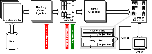
Figure 3.1: A short overview of the mesh generation process.

3.1 Marching Cubes:

As a basic visualization algorithm Marching Cubes [1] was used, which builds an isosurface on a layer of the object where a certain value of density, which is called the threshold, is assumed.

The algorithm is based on 256 cases of how a cube of 8 density values can be intersected by the surface. Each of the 8 values can be either higher or lower than the threshold. This results in 2⁸ = 256 possible combinations. In the original algorithm 15 basic cases are defined. All the other 241 cases result from either rotating or inverting a basic case.

For each of the basic cases it is shown, how the cube has to be triangulated. This triangulation is defined in a way that data values, which are higher than the threshold are separated from the others by the surface. Data values that are higher than the threshold are meant to be inside the visualized object, the others are outside.

It is commonly known that this algorithm has one major disadvantage. In some cases it is not decidable, how the triangulation has to be. A good illustration for this problem is case 13 (see figure 3.2).

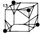
Figure 3.2: The basic case 13 featuring ambiguous faces on every side.

As mentioned above the inverted case is triangulated in the same way as the original one. In the case of basic case 13 the inverted case is the same as the case resulting from one rotation in any direction. But through any rotation the triangulation changes, through inversion it does not. Therefore it is not sure, whether to triangulate according to the inverted case or to the rotated case.

The core of the problem are the so-called ambiguous faces. A marked point represents a point with an assigned density values higher than the threshold. This point therefore is meant to be located inside the object. An ambiguous face has two diagonally opposite grid points marked and the other two diagonally opposite grid points unmarked.

There are two possibilities of how to split an ambiguous face. Either the two unmarked points are each separately isolated from the two marked (see figure 3.3 left), or the two marked are each separately isolated from the unmarked (see figure 3.3 right). In other words in the first case the two marked points are assumed to belong to the same object and in the other case it is assumed that each marked point belongs to a separate object. Of course this assumption is made from the local point of view and does not exclude the possibility that these two objects are connected elsewhere.

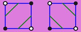
Figure 3.3: Marching Cubes, basic 2D ambiguity cases

In basic case 13, as can be seen, possibility 2 is used, in the inverted case 13 possibility 1 is used. Now, if two ambiguous faces, of which one uses possibility 1 and the other uses possibility 2, happen to face each other, the triangulations will not match and holes in the surface will be the result.

It should have become clear that the reason for those so called ambiguity cases is the fact, that inversion of a case does not change its triangulation. To solve this problem a modification of the Marching Cubes algorithm introduced by Shoeb in the year 1998 was used [2]. It consists of 8 “extra” basic cases, which cover the complementary cases to the classic basic cases, so inverted cases are no more assumed to be equivalent, which eliminates the problem. The extra cases are shown in figure 3.4.

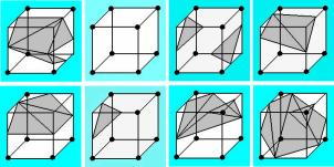
Figure 3.4: The eight Marching Cubes “extra cases”

As figure 3.5 illustrates, the 8 extra cases brought tremendous improvement.

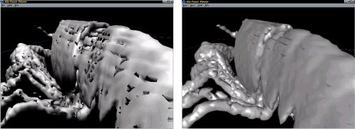
Figure 3.5: Marching Cubes without the usage of extra cases (left) and with the usage of extra cases (right). The lobster data set is courtesy of AVS inc.

3.2 Macrocubes

When processing a big data set the marching cubes algorithm produces an enormous number (usually some millions) of triangles. On a 313x313x380 metal foam data set, for example, the program generated 8 884 916 triangles. It is understandable that rendering so many triangles on a standard PC workstation results in frame rates, which are not acceptable.

One solution to that problem is to render only the necessary part of the generated triangles in every frame. To make this possible, the program divides the scene into so called macrocubes.

One macrocube consists of a user-defined number of cubes in each of the three dimensions (see figure 3.6). The advantage is that not all macrocubes have to be rendered. This will be discussed in detail in chapter 5.

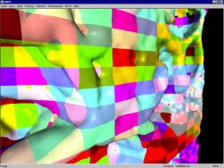
Figure 3.6: Macrocubes sized 10x10x5 cubes, painted in different colors.

3.3 Segmentation of objects.

First a definition has to be given, what an object is. One possible definition is the set of triangles connected to each other. In this paper this method is called surface segmentation. Another possibility is to define an object as the sum of triangles coating the object. In this case also two sub methods can be found. Either all triangles attached to a cell belong to the same structure or all triangles of an object belong to the same structure. The first method is called cell segmentation and the second object segmentation. Note that in general all of these methods generate a different result. This can be seen in figure 3.7.

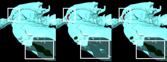
Figure 3.7: cell, object and surface segmentation (from left to right). The differences are marked with frames.

3.3.1 Surface segmentation

During mesh generation some temporary information had to be introduced. For instance a pointer to different object information structures was stored for each vertex. The fact that every triangle exactly belongs to one object can be used:

I. Generate a new triangle using the Marching Cubes algorithm.

II. Check if one or more vertex already belong to an object.

III. According to the amount of different vertices:

a. If no vertex is associated to an object, then a new object has to be generated and all vertices belong to this object.

b. If one or more vertices are already associated with the same object, then the other vertices have to be connected to this object.

c. If one or more vertices belong to different objects, then the objects have to be merged.

IV. Continue at step I. as long as there are new triangles to be generated.

V. Do post-processing on objects (i.e.: remove temporal information)

If the data set causes n triangles to be generated, the complexity is O(n) because every triangle has to be processed once and the effort for each triangle is constant.

3.3.2 Object/cell segmentation

In contrast to surface segmentation triangles need not necessarily be connected to each other to belong to the same set. (See figure 3.7). Therefore the sole mesh information is not enough to implement an efficient algorithm to segment structures. In order to solve this problem the density information and the triangle information have to be combined.

The grid of density values is traced through from the left to the right and top to bottom as can be seen in Figure 3.8. Two main steps are processed to segment the data set: (all following operations are only done if the corresponding density value is above the threshold)

I. If the neighbor on the left or top side belongs to a structure, the associated information will be used. Otherwise a new structure will be created. In both cases the vertices near this density value are inserted in this structure. If top and left neighbor are different, then a merging operation has to be applied on these.

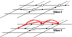
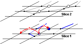
Figure 3.8: Tracing within slices in order to decide when to use existing object information. The white circles are indicating density values higher than the threshold. All small black circles showing an assumed interpolated vertex.

II. Because the data set is worked on slice by slice the new slice takes all previously determined structures if the density value is above the threshold. This step is shown in Figure 3.9. After this step the algorithm continues with step I.

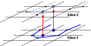
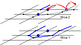
Figure 3.9: Taking information from previous slices into account when continuing with the succeeding slice.

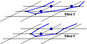
Figure 3.10: The result of object segmentation.

Cell segmentation is analogous but a little bit more complicated. Due to the Marching Cubes cases cells can also be connected through diagonals. This fact has to be taken into consideration.

In case of merging two segments all pointers to the information container of the disappearing segment have to be changed to the new one. To give the reader an insight to the problems the authors had concerning computing time it was not possible to trace the whole grid whenever a merging case arose. The impact on the performance is disastrous. For this reason all associated density points had to be stored in a separate structure in order to have direct access to the inflicted density values.

The complexity is related to the dimension of the data set. If n density values are given the complexity is O(n + plus merging overhead).

3.4 Triangle strips

Triangle strips are an efficient representation of triangle meshes. They are supported by OpenGL, which does the rendering of triangle strips much faster than the rendering of meshes represented in the standard way.

Figure 3.11 shows a small part of a triangle mesh and the order of the vertices in an ideal triangle strip.

However, such an ideal strip is not very realistic. When constructing a triangle strip, soon problems will arise. Figure 3.12 shows the same mesh as figure 3.11, but this time the vertices of the first triangle in the strip were ordered in a way, such that a problem arises when adding the last triangle.

Because one of the two vertices (2,4) which are shared between the second and the third (the rightmost) triangle, which is the new one, is not among the two last vertices (3,4) in the strip at that time. So this vertex (2) has to be added to the strip one more time (5), before the new vertex can be added (6). Figure 3.12 shows one possible way to do this.

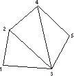
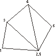
Figure 3.11: An ideal triangle strip Figure 3.12: A realistic triangle strip

The problem with that solution is, that the triangle in the middle will be represented twice in the strip, which results in an additional triangle being rendered. A better solution is shown in figure 3.13. Here the additional triangle (2,3,4) has an area of 0. Such a result can be achieved, if the new active triangle is searched already before the last vertex of the current active triangle is added to the strip, as it might be necessary to add the first vertex of the active triangle a second time before the third.

It is a good strategy to always choose the triangle adjacent to the old active triangle, which has the fewest neighbors as a new active triangle [3]. It is easy to see that this strategy dramatically reduces the possibility of triangle strips, that only consist of one triangle, and therefore extends the overall average of triangle strip length.

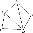
Figure 3.13: An efficient realistic triangle strip

The algorithm takes a list of triangles as input and generates a list of triangle strips as output:

I. Choose a triangle from the list and make it the active triangle.

II. Add two vertices of the triangle to the current strip, save the third one.

III. Search the neighbor of the currently active triangle, which itself has the fewest neighbors in the triangle list and make it the best neighbor. If the active triangle does not have any neighbors in the list, go on with step IX.

IV. Check, if the last vertex added to the strip (the second one of the active triangle) is part of the best neighbor. If it is, add the saved vertex (the third one of the active triangle) to the strip. If it is not, add the last but one vertex of the strip to the strip once more.

V. Delete the active triangle from the list.

VI. Make the best neighbor the active triangle.

VII. Save the third vertex of the active triangle (do not add it to the strip, just save it).

VIII. Go on with step III.

IX. The strip cannot be continued. Add the saved vertex to the strip.

X. Add the strip to the list of strips, make a new strip the current strip and move to step I.

As can be seen in figure 3.14 triangle strips do not cross macrocube borders. The reason for this restriction was the need to combine the concept of triangle strips with the macrocubes approach.

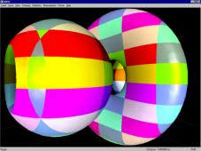
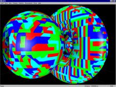
Figure 3.14: The combination of triangle strips and macrocubes.

3.5 Memory management

Because of the immense data size the authors were forced to take care of the memory usage. Running out of RAM causes the system to swap parts of the main memory to disk. When observing the memory usage a significant deviation to the estimated memory requirements could be discovered. Tracking down the problem memory fragmentation could finally be discovered guilty for this discrepancy. As shown in Figure 3.15 no memory management causes an up to three time higher memory consumption.

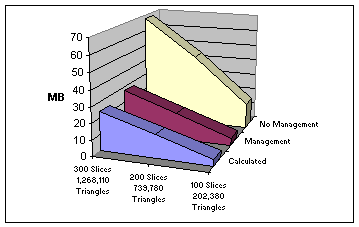
Figure 3.15: Memory usage of the program

The program uses temporal and permanent data structures. When both types are stored in the same area, they interfere with each other and cause small holes which can not be used by other data structures. See related literature for more details [5].

A workaround strategy has been developed. The system is forced to store different data-types in different locations. This is implemented using very large arrays which are managed in linear lists. Comparing the peak memory usage to the final amount of required memory a significant improvement in the amount of released memory can be noticed (see Figure 3.16).

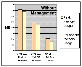
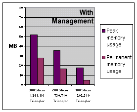
Figure 3.16: “Memory recycling” rate.

4. Interaction

Due to the requirement of a highly detailed visualization the application of levels-of-detail approaches was not possible. Therefore the following method was introduced.

4.1 Progressive rendering

As stated in section 3.2 the concept of macrocubes makes it possible to draw only the significant part of the scene during rendering of each frame in order to reduce the rendering overhead.

In fact only triangles in those macrocubes are rendered, which lie “in front of” the virtual camera and are part of the current viewing frustum. This, however is not sufficient to improve performance to interactive frame rates. That is, why another concept, the progressive rendering, was utilized.

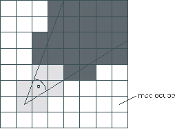
Figure 4.1: Light gray: interactive step, dark gray: completion step, white: not rendered

Peak performance of rendering is more important during periods of movement, i.e. when the virtual camera either moves through the structure or changes the viewing direction. When the camera stands still there is enough time to render the entire (or at least most of) the scene. So rendering was divided into two phases, the interactive phase and the completion phase. During the interactive phase only macrocubes within a limited environment of x macrocubes in each direction from the viewing point are tested, if they are inside the viewing frustum, and, possibly, rendered.

During the completion phase the rendered part of the scene is progressively enhanced until it comprises all the macrocubes inside the viewing frustum. The concept of progressive rendering is illustrated in figure 4.1.

4.2 Rendering

Rendering is entirely left to OpenGL, which has the functionality to map a substantial number of polygons to a hardware z-buffer in very short time [6]. The advantage of using this standardized interface is the high compatibility to most of the graphics accelerator devices.

5. Results

Figure 5.1 shows the preprocessing time of the Marching Cubes algorithm and the two main segmentation types. Additionally the amount of triangles is showed as a separate line. The analysis was done on a PII 350 MHz System with 196 MB of main memory and Microsoft Windows NT4.0 with Service Pack 5. Six different resolutions of the same data set were used in order to ensure comparable data structures.

In the case of 9 Mio. triangles the system ran out of main memory thus a serious performance degradation can be detected. The main reason why cell segmentation does not scale that good with the triangle count as the surface segmentation is that the complexity of cell segmentation is related to the count of density values and the merging operation is slightly more complicated. The relationship between density values and triangles in this data set is shown in figure 5.2.

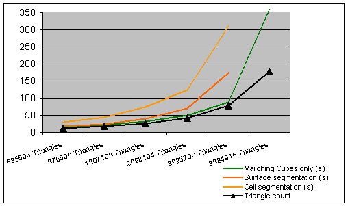
Figure 5.1: An overview of the startup time relationship

Array of density values	Triangles	MB	Marching Cubes (s)	Surface segmentation (s)	Cell segmentation (s)	Marching Cubes rate	Surface segmentation rate	Cell segmentation rate
089x089x108	635606	28	17	19	31	37389	33453	20503
104x104x126	876500	34	22	25	45	39841	35060	19478
125x125x152	1307108	42	32	40	75	40847	32678	17428
156x156x190	2098104	60	50	70	125	41962	29973	16785
208x208x253	3925790	98	88	175	310	44611	22433	12664
313x313x380	8884916	208	360			24680

Table 5.1: Startup analysis: The rightmost columns indicate the average triangle count per second.

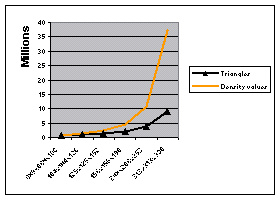
Figure 5.2: The amount of density values increases faster than the amount of triangles.

Another task was the visualization of different properties. In figure 5.3 for example the location of cells with different surface size is visualized. Furthermore detailed information related to a cell can be shown. OpenGL-supported picking is used. So a simple double click on one of the cells opens an information dialog or paints the cell in the desired color.

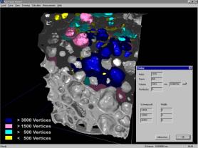
Figure 5.3: Cells of different size painted in different colors; detailed information to the white cell

In order to investigate the structure of metal foam a measurement for the quality of a cell has to be introduced. In figure 5.4 the one hundred ‘nicest’ cells are painted green, where else the one hundred worst cells are painted red. For the pictures in color please refer to http://www.cg.tuwien.ac.at/studentwork/CESCG-2000/ANeubauerAKanitsar/.

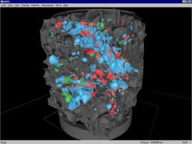
Figure 5.4: The green cells indicate a good form factor, the red ones a rather bad one.

The progressive rendering option was introduced to keep interactivity and to manage the huge amount of triangles. When investigating the interior of the aluminum foam the drawbacks of this method are marginal as can be seen in figure 5.5.

Figure 5.5: Progressive rendering: Left picture shows the interactive phase. The completion phase starts about 100 ms after movement and the final state is reached after 400 ms (right most picture).

6. Conclusion

Many of the methods we described turned out to be very helpful to satisfy the requirements risen by material scientists. The macrocubes concept restricts the complexity of rendering a scene to a nearly constant effort. This allows data sets of arbitrary sizes to be examined interactively. The progressive rendering feature eliminates the drawbacks of rendering only the local environment. Using triangle strips boosts rendering performance significantly.

Surprisingly memory management proved to have a significant impact on memory consumption. Indirectly memory usage has also an impact on performance and therefore this improvement is very important.

Some approaches developed in the scope of this project were even included in a commercial application for medical healthcare service.

7. Acknowledgements

Special credits go to Andreas König and the rest of the Institute of Computer Graphics for the support during development, implementation, and analysis of the program. The authors would like to thank Brigitte Kriszt and Andreas Kottar for the generation and provision of different data sets and feedback. Thanks also to Rainer Wegenkittel from Tiani Medgraph, Vienna, http://www.tiani.com for the inspiration he provided and the help with OpenGL details.

8. References

[1] Cline, Lorensen.: Two algorithms for 3D construction of tomographs , Medical Physics, 15 (3), pp. 320 - 327, June 1988

[2] Shoeb.: Improved marching cubes, http://enuxsa.eas.asu.edu/~shoeb/graphics/improved.html, 1998

[3] Evans, Skiena, Varshney.: Optimizing Triangle Strips for Fast Rendering, State University of New York at Stony Brook,1997

[4] Garland, Heckbert.: Surface Simplification Using Quadric Error Metrics, SIGGRAPH 97 Proceedings, Annual Conference Series, pp. 209 - 214, 1997

[5] Stroustroup.: C++ Programming Language, Addison-Wesley Publishing company, ISBN 0-201-88954-4, 1997

[6] Segal, Akeley.: The OpenGL Graphics System: A Specification, Silicon Graphics Inc., 1999

[7] Bourke, Minimum requirements for creating DXF file of a 3D model, Auckland University in Auckland, New Zealand, March 1990