Internet-Based Visualization of Basin Boundaries
for Three-Dimensional Dynamical Systems
Bernd Wallisch
Institute of Computer Graphics
Vienna University of Technology
Vienna / Austria
Abstract
1. Introduction
2. Surface Extraction
2.1 Binary
Classified Cells
2.2 Generally
Classified Cells
2.3 Surface Smoothing
3. Adaptive Surface
Representation
3.1 Adaptivity
Criteria
3.1.1
Heuristic Curvature Estimation
3.1.2
Consistency Criteria
3.2 Progressive
Refinement
3.3
Efficient Geometry Representation for Storage and Transmission
3.4
Surface Construction Algorithm
4. Domain
Boundary & Cutting Plane Preview
5. Web-Based Application
6. Results
7. Conclusions
Acknowledgments
References
Abstract
One application of surface-oriented visualization of volume data is
the construction of surfaces between two different regions of the volume
(e.g. iso-surfaces). For some applications, a binary subdivision of the
volume is not sufficient, for instance for the representation of basin
boundaries in the phase space of dynamical systems. Basins describe regions
with the same long-time behaviour. An extension of the known Marching Cubes
algorithm is introduced, which works both with binary and generally classified
(at least three different classifications within a cell) data sets. For
faster surface construction the original look-up table of the Marching
Cubes algorithm is used. The algorithm supports both progressive refinement
of surfaces by binary subdivision of data cells and smooth transitions
between models, which are differently refined. The adaptive subdivision
depends on the local properties of the surface. Binary subdivision for
refinement of regions leads to a coarse representation of the surface,
therefore the vertices of the triangles are relocated after the surface
construction depending on the classifications of adjacent cells, in
order to smooth the surface.
Keywords: dynamical systems, non-binary
classification, adaptive representation
1. Introduction
An application of surface-oriented
methods for volume visualization is the visualization of surfaces separating
distinct regions of the volume. This technique is mostly based on binary
classification of data samples in an inside and outside part by an iso-value,
i.e. the separation of data sets by a surface into two different regions
depending on a classification. But there are also applications where the
classification into more than two different regions (general classification)
is required. Nielson et al. [16] mention the segmentation of different
tissues or organ classes for medical applications or materials classified
by properties like solid, liquid or gas for physical simulation. A visualization
of more than two different regions is also required for the exploration
of boundaries between basins within dynamical systems, for example the
system discussed by Agiza et al. [1]. This application is the main motivation
for the presented project, but the surface extraction technique can also
be applied to other data sets with a binary or general classification.
The basin boundaries of a dynamical system can be considered as surfaces,
which separate regions with different long-time behaviour [17]. The problem
with dynamical systems in this context is an expensive classification function
(iteration of a trajectory) and that these classifications do not support
further information about the position of the boundary.
Following requirements for basin boundary visualization can be listed:
Fast surface construction for generally
classified regions [4, 11, 16]
The
surface construction has to be fast both for binary and generally classified
regions. The construction should only have local influence to support progressive
refinement, since new points are gradually inserted.
Adaptive and efficient model representation
[3, 10, 13, 15, 18, 24]
Because
of expensive classifications we have to use a representation with as few
as possible classified points, i.e. we use more points for regions with
a higher level of detail and fewer points for regions with a small level
of detail. Further we have to store and reuse classified points. The classification
and the surface model have to be stored in a compact way, because of the
expected high amounts of data.
Selective and smooth progressive refinement
We
have to provide the possibility of selection criteria for progressive refinement
and a high number of intermediate representations. For the selective refinement
the user is able to choose a region of interest by the actual view direction.
The selected region is first considered for refinement and is visualized
with a higher level of detail than its surrounding. Other regions are considered,
if the refinement of the selected region to the currently highest level
of detail is finished.
Web-based interactive application [7,
8, 9, 14]
The use of the Internet
is also connected with a limited bandwidth for data transmission, so we
have to reduce the data required to describe a model as far as possible.
Therefore a compact data representation for the transmission is necessary
and only the changes between different models with increasing level of
detail are transmitted.
The basin visualization
is implemented in the platform-independent programming language Java (JDK
1.2) with its 3D-extension Java 3D (Java 3D 1.1.1 Beta 1 for Direct X)
which can be used for providing 3D-graphics over the Internet [20].
2. Surface Extraction
There are only few approaches
for the visualization of generally classified data sets. These approaches
are not adequate for our application because of a subdivision of generally
classified cells in many sub cells for a generalized Marching Cubes [11]
or the use of tetrahedra for the surface construction in [4, 16]. Therefore
a modified Marching Cubes algorithm [6, 12] is used. The progressive refinement
is realized by a subdivision of a cube into 8 equally sized sub cubes.
Different levels of detail are extracted depending on the local curvature
by different subdivision depths.
The visualization of
generally classified regions requires also double-sided triangles with
different front and back side colors. Double-sided triangles can be implemented
with Java 3D using two triangles with opposite normal vectors, opposite
vertex order, activated backface culling and different colors.
2.1 Binary Classified
Cells
The original Marching
Cubes algorithm classifies the eight vertices of a cell depending on their
data value and an iso-value as inside (0) and outside (1). Every differently
classified edge of a cell contains an intersection point. The intersection
points are points of the surface, which have to be connected for triangulation.
Exploiting symmetry 15 basic cases can be identified out of 256 possible
classifications of the 8 cell vertices. The 15 cases can be stored in a
fast look-up table. The exact position of a point on an intersected edge
is calculated by linear interpolation between the two vertices using iso-value.
The normal vector on a surface point is calculated using central differences.
The Marching Cubes algorithm is reused for binary cells (exactly two different
classifications within a cell) with some modifications. For the classification
of a vertex the classification function is used, which returns which basin
a point belongs to. As only classification information is available, we
can also not calculate the position of the surface point and the normal
vector with the original methods. The position of a point is always located
in the middle of an edge, since we have no information about the exact
position from the surrounding classifications. This leads to coarse surfaces,
which can be improved with surface smoothing. A more accurate position
of a surface point can be estimated by checking the classifications along
an edge, but it is more costly. The normal vector of a point is calculated
from the location of the corresponding triangle, resulting in a single
normal vector per triangle. This is sufficient information for flat shading,
which is also sufficient for the basin boundary visualization.
2.2 Generally Classified
Cells
For the triangulation
of generally classified cells (more than two different classifications
within a cell) the cell is disassembled into several binary classified
cells. These binary cells contain only vertices with identical and adjacent
classifications from the general cell, the remaining vertices are assigned
to a so-called not defined region. These binary cells are independently
triangulated with the modified Marching Cubes algorithm. The triangulation
of a general cell is the combination of the triangulations of its binary
dissection. This triangulation approach for generally classified cells
raises the problem of not defined regions and duplicate triangles. Not
defined regions are visible at lower resolutions, but are nearly invisible
at higher resolutions. On the other hand their appearance informs the user,
that more detailed information on the junction of several regions is not
available. The duplicate triangles are caused by opposite but similar Marching
Cubes cases at the boundary. The duplicate triangle has to be removed and
the colors of the opposite triangle have to be updated. The advantages
of this method are a fast surface construction because of the reuse of
the Marching Cubes look-up table and its simplicity. Figure 1 shows an
example for the surface construction of a generally classified cell with
the modified Marching Cubes. The example leads also to a duplicate triangle.
 Figure 1 Example of general triangulation with duplicate
triangle
2.3 Surface Smoothing
Figure 1 Example of general triangulation with duplicate
triangle
2.3 Surface Smoothing
The
results of the modified surface extraction are coarse, since the vertices
are always located in the center of an intersected edge. The shape of the
surface around a vertex is influenced by the positions of other vertices.
Therefore a vertex can be relocated depending on the surrounding classifications.
A vertex on an intersected edge is influenced by the vertices in cells
sharing this common edge. Parallel edges have only a small influence, because
they do not attract connected triangles (Figure 2a). Orthogonal edges attract
triangles in their direction and cause higher curvature at the considered
vertex (Figure 2b). This attraction has to be compensated in order to get
a smoother transition. Therefore the vertex is shifted in the direction
of an intersected edge. Two intersections in different directions neutralize
each other, since every intersection is connected with relocation in its
direction (Figure 2c). Each edge is connected with 4 cells and is influenced
by 8 edges, 4 in positive and 4 in negative direction. The shift for an
edge is relative to the sum of the intersections with a sign depending
on their direction. The shift for an edge can also be scaled by a user-definable
factor in order to adjust the influence. This approach is a fast and simple
method to smooth the surface influenced by the surrounding classifications.
 Figure 2 Principle of Surface Smoothing
3. Adaptive
Surface Representation
Figure 2 Principle of Surface Smoothing
3. Adaptive
Surface Representation
The specified requirements
like adaptive representation and progressive refinement are supported by
an octree as a hierarchical data structure. An intermediate node with 8
child nodes represents every subdivision. The root node represents the
whole data set as a cube. Therefore we have to transform the data set,
since it has usually not the same extent in all dimensions. The data set,
which has to be continuously defined in the domain, is transformed by scaling
and translation into a cubic domain with the range 0 to 2^n. This domain
makes both an easier subdivision and a fast calculation with just integer
arithmetic instead of floating point possible. The cubic domain is used
for the whole work within the octree like subdivision, surface construction,
surface smoothing and so on. The domain is transformed into a domain with
the original size relations for rendering. For efficiency the octree is
replaced by an octree forest to achieve a minimum starting subdivision
and in order to avoid the traversal of these first levels. The octree forest
is a three-dimensional array (currently 8x8x8) with references to the corresponding
root nodes of shorter octrees.
The classifications of
the vertices have to be stored for reuse, because of expensive classification
functions. The storage in an array is inefficient, because of the adaptive
representation. Therefore the classifications are stored within the cell
in a compact way. For efficiency several types of leaf nodes are distinguished.
There are simple and complex leaf nodes. A simple leaf node has the same
classification at all vertices and contains therefore no surface. Most
of the leaf nodes are simple leaf nodes and can be stored with only one
classification. A complex leaf node contains at least two different classifications
and therefore a part of the surface. A complex node can be further subdivided
into binary and general leaf nodes. A binary (leaf) node contains exactly
two different classifications, so we can store them with just two classifications
and the corresponding Marching Cubes case index. All classifications have
to be stored just for the general node with at least three different classifications.
A complex node stores also a surface index to the triangles constructed
within the cell for later replacement during progressive refinement. The
distinction between different leaf node types results in big savings, since
usually at least 90% of the leaf nodes are simple or binary leaf nodes.
Simple nodes are not
further refined, since this would usually only result in more simple nodes.
This method leads to savings because of fewer subdivisions and less memory
consumption, but also to missed surface parts. Missed parts of a continuous
surface can be found by surface tracking. For surface tracking all simple
neighbours of a newly subdivided cell are checked. If a considered cell
has an intersected edge, which is adjacent to the checked simple cell,
also the simple cell must contain this intersection point and a surface
part. Therefore such simple cells are subdivided until they have the same
size as the considered cell. This method is restricted to surface parts,
which are connected to surface parts already found, which is in most cases
sufficient.
A drawback of an octree
is a difficult or expensive access to neighbour cells of the current processed
region. Therefore the leaf nodes of an intermediate node of the octree
are stored in a three-dimensional array, which works like a cache for leaf
nodes in a part of the octree. Every entry of the array refers to the corresponding
leaf node. The number of entries for a leaf node depends on its size, therefore
larger cells are represented by more entries than smaller ones. Further
for every cell the reference point within an octree, the cell size respectively
octree depth, the parent node and the child index are stored. This information
is implicitly stored in the octree and can only be determined by an expensive
traversal. The selection of the size of this array is essential for the
efficiency, since only a part of the octree can be held in this cache.
Therefore the array size is chosen to correspond to a progressive unit,
an entity used by this approach for progressive refinement.
3.1 Adaptivity Criteria
The goal of the adaptive
representation is to represent sections with a level of detail, which depends
on the local shape (curvature) of the surface. Therefore fast heuristic
curvature estimation is used as well as consistency criteria, which guarantee
a simple and fast triangulation and connection between adjacent cells with
different sizes.
3.1.1 Heuristic
Curvature Estimation
A more exact calculation
of the curvature is expensive, because we have to calculate the angles
between normal vectors of triangles of the investigated and adjacent cells.
The curvature of the cell is related to the angle between own and adjacent
triangles. This principle is reused, but every cell has only one representative
normal vector. The curvature is now estimated by the minimum angle between
the representative normal vectors of the considered and the adjacent cells.
The representative normal vector of a cell is the average or normalized
sum of the normal vectors of the vertices. The normal vector of a vertex
is calculated by the technique for discrete surfaces from Thürmer
et al. [21]. Vertices belong to the same surface, if they have the same
classification and are not separated by other classifications.
3.1.2 Consistency Criteria
The
consistency criteria guarantee a simple and fast connection between cells
with different sizes and a compact representation, since this is a common
problem for all adaptive approaches. The criteria do not have to be considered
for cells, which have only direct neighbours with the same size, since
a valid triangulation is possible with the Marching Cubes algorithm. For
the check of the consistency criteria the 6 faces of a cell are considered.
The different parts of a cell face with smaller neighbours are shown in
Figure 3.
 Figure 3 Face part designation of a cell face with smaller
neighbours
Figure 3 Face part designation of a cell face with smaller
neighbours
A non-empty cell has to be
subdivided, if any of the following rules is met.
The depth difference between the cell and a non-empty edge neighbour is
larger than 1.
The cell cannot be triangulated neither with the Marching Cubes algorithm
nor as an adaptive cell.
The faces of the cell contain more than two different classifications.
A cell is valid for Marching
Cubes triangulation, if all faces
contain no intersection point at an inner edge.
contain at most one intersection point at each border edge.
A cell is valid for adaptive
triangulation, if all following rules are met.
At most 4 faces of 6 have intersection points.
Every inner or border edge contain at most one intersection.
Every face contains either 2 or no intersections at border edges.
Every sub face contains either 2 or no intersections.
The task of the adaptive
triangulation is to connect the surfaces of adjacent cells, if the Marching
Cubes algorithm cannot be applied. The closest intersection points on the
faces of such a cell are connected in order to obtain a contour. The consistency
criteria guarantee a closed contour, so the contour can be easily triangulated
for surface construction. Figure 4 shows an example of an adaptive triangulation
of a cell with smaller neighbours.
 Figure 4 Example of an adaptive triangulated cell
3.2 Progressive Refinement
Figure 4 Example of an adaptive triangulated cell
3.2 Progressive Refinement
The principle of the
progressive refinement is to generate intermediate models with increasing
level of detail for viewing during the creation of more accurate data.
The progressive refinement is supported by a successive subdivision and
an adaptive representation. There are two combined types of progressive
refinement, smooth and selective refinement. Smooth refinement generates
many different models with different levels of detail in order to make
smooth transitions between the models possible. The selective refinement
chooses a new region in the octree for the next refinement depending on
the current view direction. All changes in this section, the so-called
progressive unit, and in adjacent cells are transmitted in one update.
The progressive unit is a cube, which corresponds to an intermediate node
of the octree.
3.3
Efficient Geometry Representation for Storage and Transmission
The task of the geometry
compression is a compact representation of the geometry. Geometry compression
is usually lossy like in [5, 19, 22]. The discrete positions in the octree
and the limited number of positions of intersection points within a cell
make a lossless and compact representation for efficient storage and transmission
possible. A vertex within a Marching Cubes cell can be stored in a compact
way using the edge identifier, because there are only 12 edges within a
cell (4 Bits). There are also 5 Bits necessary to store the shift (32 positions)
of a vertex on the edge. The triangulation of a Marching Cubes cell can
be stored with 7 Bytes (51 Bits) for the cell information and 5 Bytes (35
Bits) per triangle. The cell information consists of the cell position,
the size respectively octree depth and the front and back side color. If
we represent the triangles by its vertex positions then we need 38 Bytes
per triangle for coordinates stored as floating point numbers or 20 Bytes
per triangle for short (2 Bytes) numbers.
The compression can be
further improved if we distinguish the compression of binary (2 different
classifications) and general cells (more than 2 different classifications).
For binary cells just one front and back side color has to be stored per
cell. For general cells one front and back side color has to be stored
per triangle. Similar savings can be achieved with adaptive triangulated
cells. There are no normal vectors compressed or transmitted, since we
calculate them from the location of the corresponding triangle at the client.
3.4 Surface
Construction Algorithm
The following pseudo
code describes the principle of the surface construction and all its connected
techniques. Details about the techniques are described in the previous
or following sections. The desired level of detail is controlled by a maximum
number of subdivisions.
Initialize
octree;
WHILE
(true)
BEGIN
IF (all progressive units refined)
BEGIN
IF (desired level of detail) stop refinement;
ELSE restart refinement;
END
ELSE select progressive unit depending on view direction;
FOR (all leaf nodes within progressive unit) /* Refinement */
BEGIN
IF ((leaf node is general node) OR
((leaf node is binary node) AND
(curvature(leaf node) >= maximum curvature))
BEGIN
subdivide leaf node;
surface tracking in non-empty children of subdivided leaf node;
check consistency with neighbours;
END
END
FOR (all leaf nodes within progressive unit) /* Surface extraction */
BEGIN
surface construction within leaf node;
surface smoothing within leaf node;
if (leaf node is on the edge of the domain)
BEGIN
construct domain boundary part from leaf node;
END
END
transmit the symbolic surface representation of changed cells;
END
4.
Domain Boundary & Cutting Plane Preview
The domain boundary visualizes
the basins on the surface between the inside and the outside of the specified
data domain. The domain boundary can be considered as the cutting planes
at the 6 faces of the cube represented by the root node of the octree.
For the construction of the domain boundary the cell faces of leaf nodes
at the border of the octree are used. A quadtree is used in order to combine
smaller homogeneous faces for an adaptive representation also of heterogeneous
cells. The domain boundary provides a better overall view of basins, since
it shows also the first region corresponding to the current viewing direction,
which cannot be recognized because of double-sided surfaces.
The exploration of data
sets makes it also necessary to generate two-dimensional intersections
with cutting planes. The creation of cutting planes is expensive, therefore
a fast cutting plane preview is supported for the selection of desired
intersection locations. The preview for orthogonal cutting planes is constructed
from the classifications in the octree. The advantages are a reuse of expensive
classifications and an adaptive representation of homogeneous regions.
For the construction leaf nodes are used which are intersected by the cutting
plane. The classifications of the closest vertices are projected onto the
cutting plane. The influence of a classification on the cutting plane depends
on the corresponding cell size. A classification has more influence in
larger cells than in smaller ones.
The basin visualization
is designed to support also the application over networks like the Internet.
A surface-oriented approach is used instead of direct volume rendering,
so the geometry have to be only once constructed and transmitted for a
data set. Since the approach is view-independent no further information
have to be transmitted over the network, if the view point changes. The
progressive refinement of the approach makes also an early, low-resolution
preview of the results possible. During progressive refinement only parts
of the geometry have to be changed, so only these changes have to be transmitted.
The normal vectors of triangles do not have to be transmitted, since they
can be calculated from the position of the triangles. The normal vectors
have to be calculated at the client, which is a drawback at slow clients.
The network traffic can also be reduced by the compact, symbolic representation
of the geometry. It has the same drawback as the savings from the normal
vector calculation, since the calculation of the necessary geometry representation
has to be performed at the client.
Image 1 shows the presented surface extraction applied on the dynamical
system Game3D [1]. The smaller basins are opaque and the larger surrounding
basins are transparent displayed.
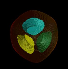
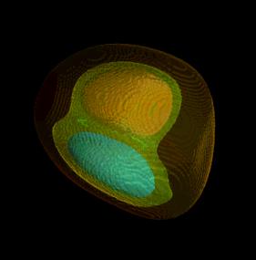 Image 1 Results of the surface extraction for dynamical system
Game3D with different parameters
Image 1 Results of the surface extraction for dynamical system
Game3D with different parameters
Image 2 shows the surface
extraction without and with activated surface smoothing for an artificial
data set. The resulting smoothed image is not completely correct, but it
is a fast approximation.
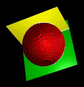
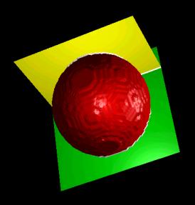 Image 2 Artificial data set without and with surface smoothing
Image 3 shows the second
dynamical system of Image 1 with a smaller function domain and a transparent
and an opaque domain boundary.
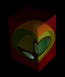
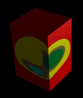 Image 3 Transparent and opaque domain boundary for dynamical system
Game 3D
Image 3 Transparent and opaque domain boundary for dynamical system
Game 3D
Image 4 shows a preview of a cutting plane through
the dynamical system Quad3D, which is from the authors of Game3D. The preview
is much faster than a calculation of the cutting plane with the same resolution.
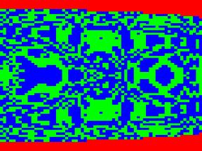
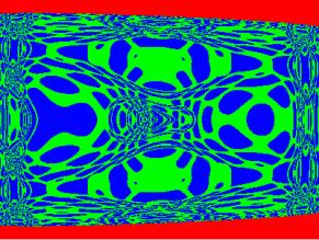 Image 4 Preview and original cutting plane of dynamical system
Quad3D
Image 4 Preview and original cutting plane of dynamical system
Quad3D
For boundary visualization of generally classified regions a modified Marching
Cubes algorithm as surface extraction technique was introduced. For triangulation
generally classified cells are subdivided into several binary cells. The
surface construction is fast, because of reusing the original Marching
Cubes look-up table. A surface smoothing method is used to smooth the coarse
Marching Cubes surface, which is caused by the selection of triangle vertices
in the center of an edge of a cell. An octree is used for adaptive representation
of homogeneous sections of the data sets. Classifications evaluated at
cell vertices by an expensive classification function are stored in the
octree in a compact way. For a better overall view of the visualization
the boundary at the border of the octree is constructed. The octree is
also used to construct a fast preview of an intersection of an arbitrary
orthogonal cutting plane with the data set in order to select interesting
locations for a cutting plane. Further information about the basin visualization
project is available at http://www.cg.tuwien.ac.at/~wallisch/da/.
Acknowledgments
Lukas Mroz, Helwig Hauser, Robert. F. Tobler, Master Eduard Gröller.
This work was supported by the BandViz project [2].
References
|
[1]
|
Agiza,
H. N., Bischi, G. I., Kopel, M., "Multistability in a Dynamic Cournot Game
with Three Oligopolists", Mathematics and Computers in Simulation 51, 1999,
pp. 63 - 90.
|
|
[2]
|
|
|
[3]
|
Bloomenthal,
J., "Polygonization of Implicit Surfaces", Computer Aided Geometric Design,
Volume 5, 1988, pp. 341 - 355.
|
|
[4]
|
Bloomenthal,
J., Ferguson, K., "Polygonization of Non-Manifold Implicit Surfaces", Proceedings
of SIGGRAPH '95, Computer Graphics Annual Conference Series, 1995, ACM
SIGGRAPH, pp. 309 - 316.
|
|
[5]
|
Chow,
M. M., "Optimized Geometry Compression for Real-time Rendering", IEEE Visualization
'97, 1997, pp. 347 - 354.
|
|
[6]
|
Cline,
H. E., Lorensen, W. E., Ludke, S., Crawford, C. R., Teeter, B. C., "Two
algorithms for the three-dimensional reconstruction of tomograms", Medical
Physics, Volume 15, Number 3, June 1988, pp. 320 - 327.
|
|
[7]
|
Elvins,
T. T., Jain, R., "Web-based Volumetric Data Retrieval", 1995 Symposium
on the Virtual Reality Modeling Language (VRML '95), ACM Press, 1996, pp.
7 - 12.
|
|
[8]
|
Engel,
K., Grosso, R., Ertl, T., "Progressive Iso-surfaces on the Web", Late Breaking
Hot Topics, IEEE Visualization, 1998.
|
|
[9]
|
Engel,
K., Westermann, R., Ertl, T., "Isosurface Extraction Techniques for Web-based
Volume Visualization", IEEE Visualization 1999, San Francisco, USA, pp.
139 - 146.
|
|
[10]
|
Grosso,
R., Greiner, G., "Hierarchical Meshes for Volume Data", Proceedings Computer
Graphics International '98, 1998, Hannover, Germany, pp. 761 - 769.
|
|
[11]
|
Hege,
H.-C., Seebaß, M., Stalling, D., Zöckler, M., "A Generalized
Marching Cubes Algorithm Based On Non-Binary Classifications", Technical
Report SC-97-05, Konrad-Zuse-Zentrum für Informationstechnik (ZIB),
1997.
|
|
[12]
|
Lorensen,
W. E., Cline, H. E., "Marching Cubes: A High Resolution 3D Surface Construction
Algorithm", ACM Computer Graphics, Volume 21, Number 4, July 1987, pp.
163 - 169.
|
|
[13]
|
Lürig,
C., Ertl, T., "Adaptive Iso-surface Generation", 3D Image Analysis and
Synthesis '96, Graduiertenkolleg 3D Bildanalyse und Synthese, 1996, pp.
183 - 190.
|
|
[14]
|
Mroz,
L., Löffelmann, H., Gröller, E., Bringing Your Visualization
Application to the Internet, Technical Report TR-186-2-98-14, Institute
of Computer Graphics, Vienna University of Technology, April 1998.
|
|
[15]
|
Müller,
H., Stark, M., "Adaptive Generation of Surfaces in Volume Data", The Visual
Computer, 9(4), 1993, pp. 182 - 199.
|
|
[16]
|
Nielson,
G. M., Franke, R., "Computing the Separating Surface for Segmented Data",
IEEE Visualization '97, October, 1997, pp. 229 - 233.
|
|
[17]
|
Peitgen,
H.-O., Jürgens, H., Saupe, D., "Chaos and Fractals: New Frontiers
of Science", Springer-Verlag, 1992.
|
|
[18]
|
Shekhar,
R., Fayyad, E., Yagel, R., Cornhill, J., "Octree-Based Decimation of Marching
Cubes Surfaces", Visualization '96, 1996, pp. 335 - 342.
|
|
[19]
|
|
|
[20]
|
|
|
[21]
|
Thürmer,
G., Wüthrich, C. A., "Normal Computation for Discrete Surfaces in
3D Space", EUROGRAPHICS '97, Volume 16, Number 3, 1997, C-15 - C-26.
|
|
[22]
|
Touma,
C., Gotsman, C., "Triangle Mesh Compression", Proceedings Graphics Interface
'98, 1998, pp. 26 - 34.
|
|
[23]
|
Wallisch,
B., Internet-Based Visualization of Basin Boundaries for Three-Dimensional
Dynamical Systems, Master Thesis, Vienna University of Technology, 2000.
|
|
[24]
|
Westermann,
R., Kobbelt, L., Ertl, T., "Real-Time Exploration of Regular Volume Data
by Adaptive Reconstruction of Iso-Surfaces", The Visual Computer, 15(2),
1999, pp. 100 - 111.
|