(1)
Jiri Walder
jiri.walder@vsb.cz
Technical University of Ostrava
Ostrava / Czech Republic
Abstract
In this article, we deal with the problem of general matching of two images taken by a camera. To find the correspondence between two images, we use the multiresolution wavelet analysis of the image functions. The wavelet analysis is good at scale adaptivity and, therefore, very effective in general image matching. We test various wavelet functions, and evaluate their reliability.
Keywords: image matching,
image correspondence, wavelet analysis
1 Two images matching
problem
2 Wavelet analysis
and image matching
2.1 Continuous
2-D wavelet transform
2.2 Continuous
wavelet transform and image matching problem
2.3 Discrete dyadic
wavelet functions
2.4 Multidimensional
analysis of the image function
f(x,
y)
3 Similarity distance
measuring
3.1 Point-to-point
similarity distance
3.2 Local parallax
continuity and generic pattern matching
4 Matching two
images
4.1 Finding exact
position in estimated neighbourhood
4.2 Spiral and
hierarchical propagation
5 Used wavelet
functions
6 Experiments
6.1 Relative gross
error
6.2 Relative gross
error RGE compared to value
LM
6.3 The resultant
parallax field
7 Conclusion
References
Suppose we have some part of a real or an artificial world. This world we call a scene. Furthermore, we suppose that objects of the scene are static. This means that they don’t move, and don’t change their shapes in time. Next we have a camera which moves in the scene. In certain short time intervals, the camera takes images of the scene.
Suppose we have two images of one scene each taken from a different position of the camera. The image matching problem refers to a process of establishing the correspondence between each pair of visible homologous image points on a given pair of images. Thus, we work with two two-dimensional (2-D) discrete image functions. In order to find the correspondence, the images have to satisfy some assumptions. Each pair of the images has no less than 50% overlapping, which is defined as the minimum ratio between the scene surface commonly depicted in both images over the surfaces depicted in each one of them. We require at least 60% overlapping, and the vergence angle formed by both image planes to be less than p /2.
2 Wavelet analysis and image matching
In this chapter, we explain how wavelet decomposition of 2-D image function f(x, y) is to be used for matching two images.
2.1 Continuous 2-D wavelet transform
A continuous 2-D wavelet transform, as a way of image decomposition, is a projection of the image function f(x, y) onto a family of functions which are linear combinations (dilations and translations) of a unique function Y(x, y). The function Y(x, y) is called a 2-D mother wavelet, and the corresponding family of wavelet functions is given by
|
|
(1)
|
|
|
(2)
|
Example of wavelet function and scale function is shown in Fig. 1. In the figure, we can also see the amplitude spectrum of the wavelet functions and the scale functions. Notice the low-pass characteristic of the scale function and the high-pass characteristic of the wavelet function.
Figure 1: Gauss wavelet function (![]() ),
scale function (
),
scale function (![]() )
and their amplitude spectra
)
and their amplitude spectra
2.2 Continuous wavelet transform and image matching problem
From previous chapter, we already know that when using the 2-D continuous
wavelet transform ![]() or the 2-D continuous scale transform
or the 2-D continuous scale transform ![]() ,
we can decompose the image function f(x,y) on different
levels of resolution (depending on the scale s). On the coarsest
level, we can easily find singularities (such as edges, corners, peaks
etc.). Then we can track them down from a high level (coarse) to the lowest
level (detail). In this way we can determine the whole correspondence between
two images.
,
we can decompose the image function f(x,y) on different
levels of resolution (depending on the scale s). On the coarsest
level, we can easily find singularities (such as edges, corners, peaks
etc.). Then we can track them down from a high level (coarse) to the lowest
level (detail). In this way we can determine the whole correspondence between
two images.
To demonstrate this point I will give you an example. Figs. 2 - 4 show the maxima of continuous Gaussian wavelet transform of two 1-D image profile functions along their homologous epipolar lines. It can be clearly seen that from the scale 32 downwards, the maxima correspondence can be easily tracked down. Homologous maxima have been determined by a naked eye, and are signed by homologous numbers. We can extend the same idea to 2-D image matching.
Figure 2: Two images of the same scene and two homologous epipolar lines
Figure 3: 1-D image functions along their homologous epipolar lines
Figure 4: Local maxima of the continuous Gaussian wavelet transform
2.3 Discrete dyadic wavelet functions
For the special class of wavelet functions, the redundant information of the continuous wavelet transform can be cleared by discretizing both the scale factor s and the translation (u, v). Strictly speaking, we will work in a dyadic wavelet space
|
|
(3)
|
|
|
(4)
|
|
|
|
|
(5)
|
|
|
(6)
|
If we use the scale function ![]() instead of the wavelet function
instead of the wavelet function ![]() ,
we get formulas for dyadic scale functions, and we will work in a scale
space.
,
we get formulas for dyadic scale functions, and we will work in a scale
space.
2.4 Multidimensional analysis of the image function f(x, y)
By multidimensional analysis of the function f(x,
y)
we understand a sequence of closed scale subspaces Vn
Vn-1![]() …
…![]() V1
V1![]() V0.
We introduce an approximation operator Aj, then Aj
f
will be an approximation of f on the jth level of resolution,
A0
represents the identity, Aj
f Î
Vj holds. The scale s on the jth level
of approximation is
V0.
We introduce an approximation operator Aj, then Aj
f
will be an approximation of f on the jth level of resolution,
A0
represents the identity, Aj
f Î
Vj holds. The scale s on the jth level
of approximation is ![]() .
Practically, we use limited number of levels j = 0, 1, …n,
where the nth level will be the coarsest resolution with the smallest
scale
.
Practically, we use limited number of levels j = 0, 1, …n,
where the nth level will be the coarsest resolution with the smallest
scale ![]() .
Next we introduce a differential operator Dj. The term
Dj
f
will denote the difference between two approximations
Aj
f
and Aj-1f
on the jth and the (j -
1)th
levels of resolution, i.e.,
.
Next we introduce a differential operator Dj. The term
Dj
f
will denote the difference between two approximations
Aj
f
and Aj-1f
on the jth and the (j -
1)th
levels of resolution, i.e.,
|
|
(7)
|
|
|
(8)
|
|
= A2 f + D2,1 f + D2,2f + D2,3f + D1,1f + D1,2 f + D1,3f … = |
(9)
|
|
|
(10)
|
|
|
(11)
|
|
|
(12)
|
|
|
(13)
|
This representation is called the wavelet pyramid of 2-D image function.
Given a discrete image f(x, y) with a limited support
x,
y
= 1, 2, …, 2n, the actual procedure for constructing
this pyramid involves computing the coefficients ![]() and
and ![]() which
can be grouped into four matrices Aj, Dj,
p,
p
= 1, 2, 3, on each level j
which
can be grouped into four matrices Aj, Dj,
p,
p
= 1, 2, 3, on each level j
|
|
(14)
|
Since we work in a discrete space, we need discrete
versions h and g of the functions f(x)
and y(x).
The coefficients ![]() and
and ![]() then
can be computed via an iterative procedure. Figure 5 illustrates the process
of the wavelet analysis. By crossing between levels j-1
and j, we first convolve the rows of the image approximation
Aj-1
f(x, y) with the discrete scale function h(x)
and the wavelet function g(x). Then we discard the odd-numbered
columns (denoted by
then
can be computed via an iterative procedure. Figure 5 illustrates the process
of the wavelet analysis. By crossing between levels j-1
and j, we first convolve the rows of the image approximation
Aj-1
f(x, y) with the discrete scale function h(x)
and the wavelet function g(x). Then we discard the odd-numbered
columns (denoted by ![]() ).
We get the approximation and the difference of given function in the
x-axis
direction. We repeat the whole process for all columns. The approximation
Ajf(x,
y)
and three difference components
Dj,p
f(x,
y),
p = 1, 2, 3 form the result.
).
We get the approximation and the difference of given function in the
x-axis
direction. We repeat the whole process for all columns. The approximation
Ajf(x,
y)
and three difference components
Dj,p
f(x,
y),
p = 1, 2, 3 form the result.
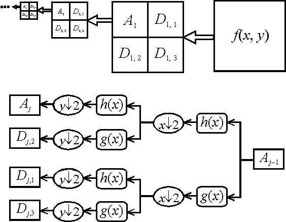
Figure 5: Wavelet pyramid and process of wavelet analysis between two levels j - 1 and j
3 Similarity distance measuring
Using wavelet analysis we can define a similarity
distance S((x, y),(![]() ))
for any pair of image points on the reference image f(x,
y)
and the matched image
))
for any pair of image points on the reference image f(x,
y)
and the matched image ![]() on any given level.
on any given level.
3.1 Point-to-point similarity distance
If we consider single point to point match on the jth level, the similarity distance can be defined using only three differential components Dj,p f(x, y), p = 1, 2, 3. For image matching to be invariant to the local image intensity, we use a normalization. This leads to the following implicit feature vector
 ,
p
= 1, 2, 3, ,
p
= 1, 2, 3, |
(15)
|
|
|
(16)
|
3.2 Local parallax continuity and generic pattern matching
For the robustness of image matching, we suppose
local parallax continuity in a neighbourhood of two integer positions (k,
l)
and ![]() ,
in another worlds, the parallax field in a neighbourhood of that two points
will be nearly the same.
,
in another worlds, the parallax field in a neighbourhood of that two points
will be nearly the same.
Let N denote the minimal neighbourhood of a given point containing the central position and four closest diagonal positions. We have
|
|
(17)
|
|
|
(18)
|
|
|
(19)
|
The generalized similarity distance ![]() is
defined as
is
defined as
|
|
(20)
|
 , , |
(21)
|
|
|
(22)
|
In this chapter, we deal with a problem of finding
full correspondence between two given images. First, we get knowledge of
finding the corresponding point if we know an approximate estimation of
its position. Next, we find approximate estimation using spiral and hierarchical
propagation.
4.1 Finding exact position in estimated neighbourhood
For any image point (k, l) in the reference
image, its approximate correspondence ![]() in the matched image may be obtained through some general strategies, such
as a spiral and hierarchical propagation to be explained later on. The
simplest way to catch the precise correspondence
in the matched image may be obtained through some general strategies, such
as a spiral and hierarchical propagation to be explained later on. The
simplest way to catch the precise correspondence ![]() is the discrete search in a small neighbourhood of
is the discrete search in a small neighbourhood of ![]() which is defined by a distance threshold Tr.
which is defined by a distance threshold Tr.
|
|
(23)
|
4.2 Spiral and hierarchical propagation
Without loss of generality, we only consider images
with size 2n ![]() 2n. By symbol Mj we denote the discrete
parallax field on the jth level of the wavelet pyramid
2n. By symbol Mj we denote the discrete
parallax field on the jth level of the wavelet pyramid
|
|
(24)
|
Each element of the parallax field ![]() contains the vector for a pair of homologous points
contains the vector for a pair of homologous points ![]() and
and ![]()
|
|
(25)
|
Gross errors of the resultant parallax field can be detected and corrected automatically by using the local parallax continuity constraint
|
|
(26)
|
After image matching on the higher (j + 1)th level, the parallax field should then be propagated to the next lower jth level. This propagation is called a hierarchical propagation. We again accurate the parallax vectors with process described in the previous chapter in Eq.(23), we search for the precise correspondence in the smallest neighbourhood of the approximate estimation of the correspondence.
All used wavelet and its associated scale functions are shown in Fig. 6. The discrete wavelet function g and its associated scale function h are mutually, therefore, we can easily compute the coefficients of the wavelet function g from the coefficients of the scale function h
|
|
(27)
|
Haar wavelets
Haar wavelets are the oldest wavelets. They are known to have the most compact support of 2, and they are orthogonal. The scale function h is
|
|
(28)
|
Daubechie wavelets (Daub-4)
Daubechie wavelets are orthogonal with compact support of 4. They are constructed to have the maximum vanishing moments. The vanishing moments of l-order are defined as
|
|
(29)
|
|
|
(30)
|
Least asymmetric Daubeshies wavelets (Symmlet-8)
They are constructed in the same way as Daubechie wavelets, but they are at least asymmetric. The scale function is
|
0.21061726710, -0.07015881208, -0.00891235072, 0.02278517294). |
(31)
|
Meyer Wavelets
They are orthogonal and symmetric, but they have no compact support. Nevertheless, for computing, the discrete version of Meyer wavelets exist. They have compact support of 62.
Symmetric complex Daubechies wavelets (Scd-4, Scd-6)
It can be shown that only complex valued scale and wavelet functions exist under the four hard conditions for orthogonality, compact support, maximum vanishing moments and finally symmetry. We denote Scd-6 the wavelet function with the shortest support of 6. It satisfies all these conditions, and it is associated with Daub-6 wavelet function. The scale function corresponding to Scd-6 is
|
|
(32)
|
|
|
(33)
|
Figure 6: Tested wavelet and scale functions
For my experiments, I chose a complex scene. I took two images of a clerical table with a digital camera from two different positions (see Fig. 2 or 11). I then used the above explained algorithm, and I experimented with different wavelet functions.
Firstly, I measured the error of bad parallax field
determination with respect to the chosen wavelet function. I measured the
difference Vj(k, l) between the
parallax vector Mj(k, l) for a given
position (k, l) with the mean parallax vector ![]() (k,
l)
in the closest 3
(k,
l)
in the closest 3 ![]() 3
neighbourhood
3
neighbourhood
|
|
(34)
|
Errors of the parallax vector Mj(k,
l)
satisfying the constraint |Vj(k,
l)|
<
LM (usually 1 ![]() LM
LM![]() 2.) can be corrected in a natural way. Nevertheless, the errors for which
the expression
2.) can be corrected in a natural way. Nevertheless, the errors for which
the expression![]() holds are gross errors, and for such errors I provided a criterion I used
for comparing the wavelet functions. The criterion of relative gross
error RGE is
holds are gross errors, and for such errors I provided a criterion I used
for comparing the wavelet functions. The criterion of relative gross
error RGE is
|
|
(35)
|
| Wavelet | RGE(M5) | RGE(M4) | RGE(M3) |
| Haar | 0.05 | 0.133333 | 0.2531 |
| Doub-4 | 0 | 0.1 | 0.24866 |
| Symmlet-8 | 0.1 | 0.125 | 0.28496 |
| Meyer | 0.05 | 0.09167 | 0.23656 |
| Scd-4 | 0 | 0.05 | 0.16578 |
| Scd-6 | 0 | 0.06666 | 0.17972 |
Table 1: Relative gross errors (RGE) on levels 5, 4 and 3
6.2 Relative gross error RGE compared to value LM
In the second test, I plotted the amount of relative gross error RGE for different values of LM into the chart (see Fig. 7 and 8).
Figure 7: Relative gross error in comparison with the value LM on 4th level of wavelet pyramid
Figure 8: Relative gross error in comparison with the value LM on 3th level of wavelet pyramid
This result shows us how large error is made by a given wavelet function. The faster the wavelet function falls the more suitable is for our use. Again, both the complex wavelet functions Scd-4 and Scd-6 are the best. From the set of the real wavelets, the Meyer wavelet function and the function Symmlet-8 are better than all others.
6.3 The resultant parallax field
As a last result, I depict resultant parallax field for the best wavelet
function, which was the complex wavelet function Scd-4. In the figures,
the parallax fields on different levels of a wavelet pyramid are depicted
by making use of a mesh. I started finding the correspondence on the 5th
level of the wavelet pyramid with the approximation of size 8 ![]() 8. The result of searching on this level can be seen in Fig. 10. The figure
on the left shows the reference image. The figure in the middle shows the
parallax field just after the initialization in the reference image. The
figure on the right shows the corrected parallax field in the reference
image corrected with the discrete search in the neigbourhood of the approximate
estimation of the correspondence).
8. The result of searching on this level can be seen in Fig. 10. The figure
on the left shows the reference image. The figure in the middle shows the
parallax field just after the initialization in the reference image. The
figure on the right shows the corrected parallax field in the reference
image corrected with the discrete search in the neigbourhood of the approximate
estimation of the correspondence).
Figure 10: Parallax field found on the highest 5th level of size 8 ![]() 8
8
Crossing from the level 5 to the level 4 with size
of 16 ![]() 16 is shown in Fig.
11, and crossing from the level 4 to the level 3 of size 32
16 is shown in Fig.
11, and crossing from the level 4 to the level 3 of size 32 ![]() 32 is shown in Fig. 12. The figure in the middle shows the parallax field
initiated just after the hierarchical propagation from the level 5 to 4
and from the level 4 to 3, respectively. The figure on the right shows
the corrected parallax field.
32 is shown in Fig. 12. The figure in the middle shows the parallax field
initiated just after the hierarchical propagation from the level 5 to 4
and from the level 4 to 3, respectively. The figure on the right shows
the corrected parallax field.

Figure 11: Parallax field found on the 4th level of size 16 ![]() 16
16
Figure 12: Parallax field found on the 3rd level of size 32 ![]() 32
32
I evaluated the found correspondence between the two images by a naked eye. At a first glance, we can see that the mentioned algorithm works very well. There are only few errors in the middle area of the parallax field. The most errors are in the border area in which the constraint of continuity of the parallax field is hard to apply. Therefore, the next improvement of this algorithm should aid at removing the errors in the border area.
In this work, I explained the algorithm for matching two images taken by a digital camera. The algorithm is based on the usage of wavelet transform. I used several of the most important wavelet functions for testing. The symmetric complex wavelet functions (Scd-4 and Scd-6) proved to be the best choice. From the set of real wavelets, we recommend to use the Meyer wavelet function. Except for the border parts, the above explained algorithm for the image matching works very well.
| [1] | Castleman, C.R.: Digital image processing, Prentice Hall, Upper Saddle River, New Jersey, 1996. |
| [2] | Castova, N.: Teaching text for seminar about Integral transforms and spectral analysis, VSB TU Ostrava, 2000. |
| [3] | Wavelet Toolbox User’s Guide by The MathWorks, http://www.mathworks.com, 2000. |
| [4] | Pan, H.: General Stereo Matching Using Symmetric Complex Wavelets, paper presented at SPIE Conference: Wavelet Applications in Signal and Image Processing IV, August 1996, Denver, USA, published in SPIE Proceedings vol. 2825. |