Simultaneous Effects of the Environment and the Tropism
to the Growth of a Tree
Ladislav
Kovács
e-mail
: Ladislav.Kovacs@st.fmph.uniba.sk
Department
of Computer Graphics and Image Processing
Faculty
of Mathematics and Physics
Comenius
University
Bratislava
/ Slovakia
Abstract
The goal of this work is to extend Lindenmayer systems in a manner suitable for simulating the interaction between a developing plant and its environment. Our tree-like model will consider two kind of interactions: a tree’s response, growing outside or inside of a sphere, to the collision with the sphere and a tropism which will cause that the branches tend to grow on the surface of the sphere. The extension of the environment is also presented as a generalization of the algorithm.
Keywords: L-systems, turtle geometry, environmentally-sensitive extension of L-systems, tropism
1. Introduction
Since a biologist, Aristid Lindenmayer, has proposed the formalizm of Lindenmayer systems, in short L-systems, as a general framework for plant development, a various kind of extension of L-systems has been arisen. Some of these, such as table L-systems, are able to model environmental factors and others, for example environmentally-sensitive L-systems and open L-systems, are capable of bi-directional simulation of interaction between a plant and its environment as it is showed in [5].
In our model environment will be represented as a sphere, so information exchange will consists of the reception of information about this sphere and the generation of the response in the form of growth changes, e.g. changes the direction of branches. In addition to this, our sphere is considered as a special solid, which acts as follows :
· If the tree grows inside of the sphere then the whole surface of the sphere is considered to be made of glass, so branches tend to grow out of the sphere in order to obtain the utmost light. This response to light is also called phototropism.
· If the tree grows outside of the tree, the sphere acts as a thermo-light-source, therefore branches try to wreathe the whole sphere. This phenomenon is known as thermotropism.
2. Basic Notions and Branching Structures
2.1
L-systems
We will use L-systems to generate our tree-like structures. There are known a lot of books about these systems, see [1] for more information and exact definitions, so let us just briefly introduce them through some frequently used expressions.
The central notion of
L-systems is the concept of rewriting. The basic strength of rewriting lies in
the ability to define complex object by successively replacing parts of
a simple initial object using a set of rewriting rules or productions.
Productions are applied in
parallel, with all letters being
rewritten simultaneously in a given word, since development of plants takes place simultaneously in all
parts of an organism.
A production consists of two
strings - the predecessor and successor. When the production is
applied to the string, the predecessor is compared against each symbol of the
string. The successor replaces the symbol in the string if the symbol matches
the predecessor.
In the process of string
rewriting the string keeps growing in length and all the patterns of the old
strings are preserved in some way. The number of times a string is rewritten is
called depth or derivation step. The first derivation starts by applying the
production rules to the axiom as the
current string. The successive strings are generated with the previous strings
as the input, and then productions rewrite the strings. Simple axioms and rules
produce strings with more and more complicated patterns, even complicated
enough to mimic nature's growing process.
2.2
Turtle
Graphics
Strings generated by L-systems may be interpreted geometrically in many ways. We use an interpretation introduced by Szilard and Quinton and extended by Prusinkiewicz and Hanan which is based on the LOGO-style turtle, where the movements of the turtle is controlled in accordance with the meanings of generated string.
2.2.1 3D Turtle Graphics
After a string has been generated by an L-system, it is scanned sequentially form left to right, and the consecutive symbols are interpreted in accordance with their geometric meanings. In 3D the state of the turtle is defined by its position and its heading vector. Let us consider letters which are interpreted by the turtle in 3D:
F : move forward a step of length defined during the interpretation and draw a defined object from the original to the new position of the turtle.
f : move forward a step of length defined
during the interpretation without drawing an object. The turtle acts as in the
previous case, but there won’t be drawn an object between the new and the
original positions. ![]()
+ : Turn right by angle defined in advance.
- : Turn left by angle given in advance.
[ : Push the current state of the turtle
(position, orientation, width and length of objects being drawn, as well as
other attributes, such as color ) onto a pushdown stack.
] : Pop a state from the stack and make
it the current state of the turtle. No object is drawn, although in general the
position and orientation of the turtle are changed.
We have to take into account, that trees are perhaps the strongest structures in living nature, so our models have to be continue enough at any branching point. In order to achieve the continuity of direction at fixed point, an interpolating cubic spline will be used to draw the branches of a tree.
According to the notations given in the figure below we can define the following expressions:
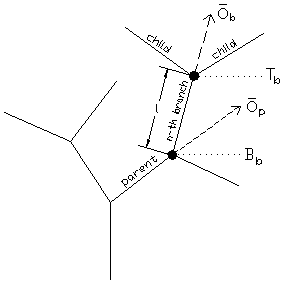
Figure 2.1: Notations in reference to the nth
branch
· Branch – an object represented by the symbol F, which causes the turtle draw;
·
Base (starting)
point of the nth branch ![]() – a state of
the turtle just before the symbol F
starts to draw the nth branch;
– a state of
the turtle just before the symbol F
starts to draw the nth branch;
·
Top (end) point of the n-the branch ![]() – a state of the
turtle after the interpretation of the nth branch;
– a state of the
turtle after the interpretation of the nth branch;
·
Orientation of
the nth branch ![]() – the orientation
of the turtle during the interpretation of the nth branch;
– the orientation
of the turtle during the interpretation of the nth branch;
·
Length of the nth
branch (l) – the distance between the start and top points of the nth
branch;
·
Width of the nth
branch (r) – a positive real number;
·
Child branch(es)
of the nth branch (child) – branch(es) which starting point(s) is (are) the
same as the top point of the nth branch;
·
Parent branch of
the nth branch (parent) – the branch which child branch is the nth branch;
·
Parent direction
of the nth branch ![]() – the orientation
of the turtle during the interpretation of a parent branch; it is used in
space model along with a divergence angle.
– the orientation
of the turtle during the interpretation of a parent branch; it is used in
space model along with a divergence angle.
Our symbols are useful to
describe the representation of a branch with a spline. All branches,
except the first one being created, is represented as a cubic spline
segment of a form: ![]() ,
, ![]() ,
, ![]() . For the nth branch the spline segment satisfies the
following symbolic conditions:
. For the nth branch the spline segment satisfies the
following symbolic conditions: ![]() ,
, ![]() ,
, ![]() and
and ![]() . By means of these formulas parameters a, b, c and d of the cubic spline segment Q
could be expressed as follows:
. By means of these formulas parameters a, b, c and d of the cubic spline segment Q
could be expressed as follows: ![]() ,
, ![]() ,
, ![]() and
and ![]() .
.
Let ![]() is a parametric form
of a circle having its centre in the point C with a radius r
and being located in a normal plane of a
is a parametric form
of a circle having its centre in the point C with a radius r
and being located in a normal plane of a ![]() vector.
A wire-frame model of a branch will be represented by solid
vector.
A wire-frame model of a branch will be represented by solid ![]() , where
, where ![]() ,
, ![]() and
and ![]() is the width of the parent branch. This solid could be
imagined as a sequence of consecutive circles which are located in
a normal plane of a vector
is the width of the parent branch. This solid could be
imagined as a sequence of consecutive circles which are located in
a normal plane of a vector ![]() with their centres
passing along the spline defined above and whose radii are changed
according to the value
with their centres
passing along the spline defined above and whose radii are changed
according to the value ![]() .
.
3.
Adding Variation to the Model
2.2
Stochastic L-systems
To avoid the artificial regularity of models generated by deterministic
L-system, variation of turtle interpretation and/or randomization of
L-productions are needed.
Randomization of the interpretation alone has a limited effect: it changes
only geometric aspects of a plant, such as the stem length and branching
angles, but the topology remains unchanged. In contrast, the stochastic
application of production may affect both the topology and the geometry of the
plant.
In this system there could
be several rules with the same matching condition. The choice of a specific
rule to apply string rewriting is determined by a probability distribution as a parameter of this set of rules. The
interesting effect of a stochastic L-system is that it will produce different
output every time, or in other words, the growth is not predictable or
reproducible with the same axiom and rules.
4. Botanical Rules and their Application in the Trees Development
The growth of a tree in the nature takes place in accordance with a couple of botanical rules. In our models we also try to take into account some of these rules.
First of all it is well known that the leaves of the branches are often arranged in such a way that leaves above do not hide leaves below. This means that each gets a good share of the sunlight and catches the most rain to channel down to the roots as it runs down the leaf to the stem. This attribute of the leaves can be used to the arrangement of the branches as well and has a very interesting connection with the mathematics as it is showed in the chapter 4.1.
Natural factors, such as the gravitation force or wind, could also affect the growth of the branches. These outer forces are called the tropism.
Just as in the nature, in our model we have to take into account
a very essential fact that the length of the branches as well as their
radii are becoming shorter and shorter as a tree grows. This natural
phenomenon can be captured by a contraction.
4.1
The Divergence
Angle
The pattern formed in the stem by the alternation of branches is affected by the phyllotaxis, i.e. arrangement of the leaves, because branches originate in the axils of the leaves, so phyllotaxis, give us information about the arragement of the branches as well.
Leaves succeed one after
another along a so-called genetic
spiral (or helix). The genetic
spiral passes through the leaves in their numerical order, that is, the order
of their production. In order to describe the arragement of the branches on the
stem, it is needed to know the angular
divergence of the leaves. The divergence angle between the leaves is given
as ![]() . By finding two superimposed leaves we can count the number
of leaves
. By finding two superimposed leaves we can count the number
of leaves ![]() and the number of
turns
and the number of
turns ![]() around the axis
between these two superimposed leaves. The fractions most frequently belong to
the Fibonacci summation series,
around the axis
between these two superimposed leaves. The fractions most frequently belong to
the Fibonacci summation series, ![]() ,
, ![]() ,
, ![]() ,
,![]() ,
, ![]() ,
, ![]() , etc., in which each value of the numenator and the
denominator is a sum of the two corresponding Fibonacci values that
precede it. This fact was discovered at the end of the nineteenth century and
is often called Schimper-Braun’s law. The amazing thing is that this single
angle enables to produce the the whole tree no matter how big the plant grows.
This principle of the divergence angle was only proved mathematically by two
French mathematicians Douady and Couder in 1993.
, etc., in which each value of the numenator and the
denominator is a sum of the two corresponding Fibonacci values that
precede it. This fact was discovered at the end of the nineteenth century and
is often called Schimper-Braun’s law. The amazing thing is that this single
angle enables to produce the the whole tree no matter how big the plant grows.
This principle of the divergence angle was only proved mathematically by two
French mathematicians Douady and Couder in 1993.
4.2
Contractions
4.2.1. Contraction of a Branch’s Length
Contraction of the branches’
length is computed as the contraction ratio of the child branch to its mother
branch. This parameter is not affected by any values and our only restriction
is that a child branch is need to be shorter than its mother branch. In
order to achieve randomness and natural looking of our model, the length’s
contraction need to be counted with a dispersion from a relatively
big interval. We assume that the contraction of a branch’s length to be ![]() , length of a parent branch to be
, length of a parent branch to be ![]() , length of its child
branch to be
, length of its child
branch to be ![]() , and a random dispersion to be
, and a random dispersion to be ![]() . To the length of the child branch the following relation
can be easily obtained:
. To the length of the child branch the following relation
can be easily obtained: ![]() .
.
4.2.2. Contraction of a Branch’s Radius
Contraction of the branches’
radius is given as the contraction ratio of the child branch to its mother
radius. Before setting the radius of a child branch, we need to take into
account one natural rule which says that a child branch is thinner then its
mother branch, i.e. radius never expands. Keeping this principle we can use the same formula used in
the previous section.
4.3
Tropism
A characteristic feature of turtle interpretation is that directions are specified relative to the current orientation. However, absolute directions play an important role in the development of plants. For example, branches may bend due to the effect of wind, sunlight or gravity. These movements can occur as a consequences of tropism.
Tropism is defined as a response or orientation of a plant to a stimulus that acts with greater intensity from one direction than another. It may be achieved by structural alteration. Forms of tropism used in our model include phototropism (response to light) and thermotropism (response to thermae).
Tropism can be classified from the point of view of mathematics into two groups:
1) according to its
kind of effect we distinguish:
a) point controllers (an effect to a plant
from one point, such as phototropism: the plant tends to bend towards the
source of light);
b) vector controllers (a plant make its movements
in a specified direction, for example geotropism: active movement along
the gravitational force)
2) according to its
orientation:
a) attractors (attraction forces - warmth and light);
b) inhibitors (repulsive forces - wind).
Vector controller has an
important role in our model, therefore let us describe
its mathematical model. If we refer to the vector controller as
a quadruple ![]() , the new top coordinate, denoted as
, the new top coordinate, denoted as ![]() , of a branch is described as shown below, where vs denotes the controller’s strength,
, of a branch is described as shown below, where vs denotes the controller’s strength, ![]() is the controller’s
vector (it is assumed to be an unit vector), BranchLength is the length of the branch,
is the controller’s
vector (it is assumed to be an unit vector), BranchLength is the length of the branch, ![]() is the direction of
the branch and
is the direction of
the branch and ![]() is the original top
coordinate of the branch.
is the original top
coordinate of the branch.
![]()
![]()
![]() .
.
Whether a controller is an attractor or an inhibitor
is determined by the sign of the strength; if ![]() it is an attractor,
consequently the tip moves along the vector
it is an attractor,
consequently the tip moves along the vector ![]() , otherwise it is an inhibitor. In our mathematical model we
assume that
, otherwise it is an inhibitor. In our mathematical model we
assume that ![]() , so we have an attractor. This method is based on the
rotation of the direction of the branch, so the length of the branch is kept
under any circumstances.
, so we have an attractor. This method is based on the
rotation of the direction of the branch, so the length of the branch is kept
under any circumstances.
5. The Algorithm
Now we describe the algorithm which is used in the generation of a tree considering the bi-directional information exchange as well as the tropism. Before the representation of the drawing symbol F in the string generated by L-system, we have to examine the branch position, because at first there have to be detected the possible obstacle (the sphere) and in accordance with this the position and orientation of the turtle should be adjusted. We also have to take into account the effect of the tropism to the branches at the same time. To summarize, our task is to reach a new position and orientation of a branch.
5.1 The Growth of a Plant Outside of the Sphere
At first we consider the
situation when a tree is growing outside of the sphere. For the sake of
simplicity we can assume that all branches are represented as a line segment.
The location and the radius of the sphere, representing the environment and
noted as ![]() , where S is the
center and R is the radius of this
sphere, is given as an input data. The following notation refers to the child
branch: B – the start point, T –
the top point, T’ – the new position of the top point.
It is assumed that the new position of the top point of the parent branch has
already counted by the algorithm described below.
, where S is the
center and R is the radius of this
sphere, is given as an input data. The following notation refers to the child
branch: B – the start point, T –
the top point, T’ – the new position of the top point.
It is assumed that the new position of the top point of the parent branch has
already counted by the algorithm described below.
We can state two rules which determine the computation of the new top position of the branch:
Ø
If any point of the branch is in the sphere then the
relocation is accomplished as follows: It can be distinguished two cases in
this situation according to the distance between points B and TangPoint, where the
TangPoint is such a tangent
point of the sphere ![]() from the point B which is closer to the point T (see figure 5.1).
from the point B which is closer to the point T (see figure 5.1).
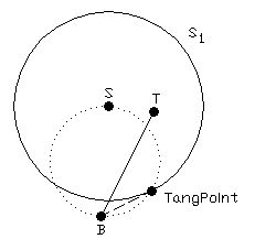
Figure 5.1: A simple test of the re-location.
If ![]() then we create a sphere
then we create a sphere ![]() and compute the
intersection circle, let us denote
and compute the
intersection circle, let us denote ![]() , of the spheres
, of the spheres ![]() and
and ![]() ,
, ![]() . In this circle we find such a point T’ which is in the closest distance from
the top of the branch. , which has to be re-located. The point T’ is the new position of the top
of the branch, because d(B,T’)
. In this circle we find such a point T’ which is in the closest distance from
the top of the branch. , which has to be re-located. The point T’ is the new position of the top
of the branch, because d(B,T’)![]() and T’ is on
the surface of the sphere.
and T’ is on
the surface of the sphere.
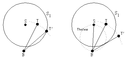
Figure 5.2: Improper re-location.
Figure 5.3: Finding the tangent point.
If ![]() then we cannot use the method described above, because it can
be happen that after the relocation of the top point of the branch some points
of the re-located branch is still in the sphere (see figure 5.2). In this case
we have to create a new sphere
then we cannot use the method described above, because it can
be happen that after the relocation of the top point of the branch some points
of the re-located branch is still in the sphere (see figure 5.2). In this case
we have to create a new sphere ![]() and repeat all the
steps as above. In this case we find the special tangent point of the sphere
from the point B which is in the closest distance from the
point T, see figure 5.3, which enable
us the determination of the new position of the top of the branch.
and repeat all the
steps as above. In this case we find the special tangent point of the sphere
from the point B which is in the closest distance from the
point T, see figure 5.3, which enable
us the determination of the new position of the top of the branch.
Ø
If all points of the line segment is outside of the
sphere then we use tropism to re-locate the top point of the branch. The vector
controller’s strength is counted as ![]() , where
, where ![]() and the
controller’s vector is a vector
and the
controller’s vector is a vector![]() , see Figure 5.4.
, see Figure 5.4.
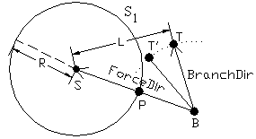
Figure 5.4: The effect of the tropism
We could reach an interesting phenomenon if we define the following rules:
Ø The attraction force of the sphere to the branches is taking into account after the branches’ width is less then a certain value
Ø Any kind of re-location is applied only if the z-coordinate of any point of the branch is grater then the minimum z-coordinate of the sphere. In this case the tree grows freely in it natural environment without obstacle until its branches doesn’t fulfil the rule. This delayed deviation causes such an effect as the sphere appears later in the vicinity of the tree then the tree starts growing.
5.2 The Growth of a Plant Inside of the Sphere
If the tree grows inside of the
sphere we could also use all the rules written above with some modification: We
have to re-locate the branches if their top points are outside of the sphere
and the tropism is taking into account when all points of any branch is inside
of the sphere. In this case the vector controller’s strength is counted as ![]() and the controller’s
vector is a vector
and the controller’s
vector is a vector ![]() (see figure 5.4),
where the point P is a common
point of the sphere’s surface and the vector ForceDir.
(see figure 5.4),
where the point P is a common
point of the sphere’s surface and the vector ForceDir.
5.3 Extension of the Environment
Environment represented so far
consists only of the sphere which is situated in the vicinity of a tree.
This very simple situation could be easily extended by adding another sphere to
the existing one. This new sphere has also an affect to the tree as the
first one. In this extension there is a possibility to set the strengths
of the attraction forces of the spheres separately. These strengths are
combined with the distance between the tree and the spheres according the
formula described later in this section. These strengths are denoted as TropismStrength and SecTropismStrength and are chosen from the interval ![]() , where 0 denotes
that the given sphere has no effect to the tree and the sphere has
a maximum affect to the tree when 1 is chosen from the interval.
, where 0 denotes
that the given sphere has no effect to the tree and the sphere has
a maximum affect to the tree when 1 is chosen from the interval.
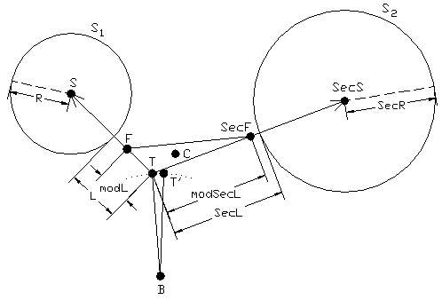
Figure 5.5: Re-location of the tip
of the branch.
At first we describe the whole re-location process, which can be used in the case when the environment is represented with two spheres, if all points of the line segment representing the branch is outside of the spheres. It is assumed that the two spheres doesn’t intersect each other.
The location and the radius of
the first sphere is noted as ![]() , where S is the
centre and R is the radius of this
sphere;
, where S is the
centre and R is the radius of this
sphere; ![]() denotes the second
sphere, where SecS is the centre and SecR is the radius of this sphere. Spheres are given as an input data. If
we refer to the figure 5.5 the following notations can be written down: B
– the base point of a branch, T – the original top point of
a branch, T’ – the new top of
a branch,
denotes the second
sphere, where SecS is the centre and SecR is the radius of this sphere. Spheres are given as an input data. If
we refer to the figure 5.5 the following notations can be written down: B
– the base point of a branch, T – the original top point of
a branch, T’ – the new top of
a branch, ![]() ,
, ![]() .
.
The first controller’s vector
is a vector ![]() and the second one is
the vector
and the second one is
the vector ![]() . If we take into account the affects of the spheres to the
point T, which has to be re-located,
and the distances of the spheres from this point then two points F and SecF can be symbolically counted as follows:
. If we take into account the affects of the spheres to the
point T, which has to be re-located,
and the distances of the spheres from this point then two points F and SecF can be symbolically counted as follows:
![]()
![]() .
.
Vectors ![]() and
and ![]() are the new
controllers’ vectors, but we need only points F and SecF in this re-location process. Values
are the new
controllers’ vectors, but we need only points F and SecF in this re-location process. Values ![]() and
and ![]() decrease with
increasing L and SecL respectively, so the sphere has as smaller affect to the
branch as it is located further from the sphere.
decrease with
increasing L and SecL respectively, so the sphere has as smaller affect to the
branch as it is located further from the sphere.
The C point is the centroid of the triangle given with the vertexes F, SecF
and T. This point C is the
reference point of the vector ![]() . The original direction of the branch is
. The original direction of the branch is ![]() . The new direction of the branch is counted as
. The new direction of the branch is counted as ![]() . The new top point of the branch can be easily determined
using this vector as follows: T’
. The new top point of the branch can be easily determined
using this vector as follows: T’![]() , where NewBranchDir is assumed to be an unit vector and
BranchLength is the length of the branch.
, where NewBranchDir is assumed to be an unit vector and
BranchLength is the length of the branch.
If any point of the branch is in any sphere then at first we determine the sphere with which the branch has intersection and the relocation after that is accomplished as it is fully described in the part 5.1.
6.
Results
In this section some pictures are presented which were generated using our algorithm.
The extension of the environment is captured in the first picture of this capture. The spheres’s location, radii and the strengths of their attraction forces are chosen to be different.
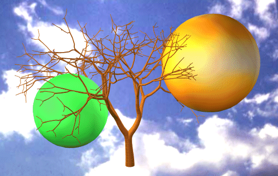
Figure 6.1:
The extension of the environment
In the figure 6.2 the tropism affects to the tree from the
beginning of the growth of the tree. It can be noticed that due to the tropism
the branches of the tree are always located near to the surface of the sphere.
Figure 6.3 shows a tree which
grow inside of the sphere. We can see that the tree starts to grow outside of
the sphere, but after its first branch get into the sphere all the branches
remain their positions inside of the sphere.
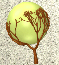
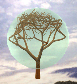
Figure 6.2: Outside of the sphere.
Figure 6.3: Inside of the sphere.
7.
Conclusion and Future Work
In this paper we presented an algorithm which could be used to the simulation of the tree’s response, growing outside or inside of a sphere, to the collision with the sphere and the tropism. We presented the environment with the sphere and we assumed the sphere to be a special object in this environment which causes the tropism. The tree is tend to reach our sphere under any circumstances because of the tropism, so to speak the sphere drags the branches towards itself.
The implementation and the result of this algorithm is the main theme of my diploma thesis. The future work will include solving the situations when the environment is represented with another sort of objects and leaves, flowers and fruits could be also added to the tree-models generated also by L-systems.
References
[1] Przemyslaw
Prusinkiewicz, James Hanah: Lindenmayer
systems, fractals and plants, vol. 79 of Lecture notes in biomathematics,
Springer verlag, Berlin 1989
[2] Masaki Aono,
Tosiyasu L. Kunii: Botanical Tree Image Generation, IEEE Computer Graphics
& Applications, May1984, pp. 10-33
[3] Norbert Filip:
Modelovanie stromov pomocou L-systémov, Diploma Thesis, MFF UK Bratislava 1993
[4] E. Ružický, A.
Ferko: Počítačová grafika a spracovanie obrazu, Sapienta 1995
[5] Radomír Měch and
Przemyslaw Prusinkiewicz. Visual Models of Plants Interacting with their
Environment. Proceedings of SIGGRAPH’98, pages 48-61, ACM
SIGGRAPH, 1998
[6] Katharine
Esau: Plant Anatomy, John Wiley & Sons, Inc., 1965