Postprocessing and Visualization of peripheral CTA data in clinical environments

Abstract

This paper deals with computed tomography angiography based vessel exploration. Large image sequences of the lower extremities are investigated in a clinical environment. Two different approaches for peripheral vessel diagnosis dealing with stenosis and calcification detection are introduced. The paper presents an automated vessel-tracking tool for curved planar reformation. A user interactive segmentation tool for bone removal is proposed.

Keywords: computed tomography angiography, semi automated segmentation, optimal path computation, vessel tracking.

1.     Introduction

Lower extremity arterial disease is a significant health problem in the industrial world. The prevalence of symptomatic disease (intermittent claudication) in patients between 55 and 74 years of age is 4.6% [3]. Nowadays, intra-arterial digital subtraction angio­graphy (iaDSA) is the pretherapeutic imaging technique of choice. iaDSA, however, is an invasive and costly procedure, which requires arterial catheterisation. A non-invasive technique for imaging the entire inflow and run off vessels is therefore desirable.

Latest technical developments in computed tomography (CT) —notably multi-slice helical CT— allow an unprecedented volumetric resolution and a widespread anatomic coverage. A multi-slice helical CT thus has the potential to accurately show the entirety of the lower extremity vessels with a single intravenous contrast-medium injection at a high, near isotropic spatial resolution.

The data acquisition time for a dataset of the lower limbs is in the range of minutes. On the other hand, the post processing time using conventional techniques takes up to four hours. However this step is necessary in order to extract useful information from the huge amount of acquired data. In order to make this investigation method applicable in the daily clinical use, the post processing time has to be shortened.

2.     Peripheral vessel investigation

Computed tomography angiography (CTA) datasets of the peripheral vessel structures belong to the largest datasets in medical imaging. Current resolution is up to 1500 slices, each slice containing 512 to 512 pixels with a depth of 16 bit. Therefore for the practicability of CTA of the lower limbs it is crucial to provide an appropriate visualization tool for vessel investigation. It turned out that this tool should have the following properties:

·      Easy and fast to handle, as the tool should be used in a clinical environment for routine purposes.

·      Adequate quality of the results, which means the results should be diagnosable.

·      Robust algorithms are required as the anatomic variations are quite large due to different vessel diseases.

Stenoses, calcifications and occlusions are the main arterial diseases that shall be investigated with CTA. A stenosis is a narrowing of the arterial flow lumen. Arterial stenoses are caused by atherosclerotic plaque (figure 1a). A complete obstruction of a vessel is referred to as an occlusion (figure 1b). The blood flow is redirected through secondary vessels, which circumvent the occluded vascular segment, and which are called collateral vessels. The vessel wall of diseased arteries, as well as atherosclerotic plaque may calcify. With CT, calcified tissue is of high attenuation. In figure 1, several areas of calcification can be seen (e.g., figure 1c).

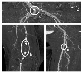
Figure 1: Different arterial diseases: Stenosis (a), Occlusion caused by calcification (b) and Calcification (c).

3.     Visualization Methods for CTA

Basically two different approaches were followed in order to provide a feasible tool for investigating CTA datasets [5]. The first is to generate a curved planar reformation (CPR). This method is already used in medical environments. Therefore, it is a visualization technique that is very likely to be accepted for daily clinical use by the medical personnel in hospitals. One of the biggest disadvantages of this technique is an extremely time-consuming and error prone manual generation process. For this reason, a semi automatic generation method is desirable. Such an approach is described in section 3.1.

The second approach is quite different. As the vessel tree in the lower extremity areas consists of a huge amount of blood vessels of all sizes it is very difficult to identify every single vessel. Nevertheless, these small vessel structures are important to a radiologist. For instance the lumen of the small collateral arteries may allow a deduction of the spatial extend of a stenosis of the main artery. The basic idea of the second approach is that if it is difficult to identify the structures of interest, it might be easier to hide structures of less or no importance. Following this approach the whole vessel tree can be made visible with a maximum intensity projection (MIP) by removing the bones from the dataset first. This method is described in section 3.2 in more detail.

It turned out that both visualization techniques are needed in order to produce results with diagnostical value. An overview of the whole vessel tree is provided by the MIP visualization. In addition to that the extend of calcification can be determined as every calcified area will be visualized in it’s entirety. Precise information concerning the vessel lumen and the extension of the stenoses are made available by the CPR visualization method.

3.1     Automated CPR Generation

Planar cross-sections through volume data are often used for investigating CTA datasets in medical imaging. This is a very circumstantially method for vessel investigation as only small parts of the vessels are visible within one planar cross-section. For this reason we want to compute a cross-section through the centerline of a vessel.

The central line of a vessel is seen as a 3D curve. A line is defined through each point of this curve, which is parallel to the horizontal axis of the viewing plane. This line is swept through the 3D curve, generating a curved plane (see figure 2). The voxels in the close neighborhood of the plane are resampled. Finally the plane is flattened and displayed in 2D. This process is called curved planar reformation (CPR).

Taking the vessel central axis as curved line for the curved planar reformation prevents the vessel from being covered by bony structures. Furthermore, the true vessel lumen can be determined in this representation even if calcified vessel walls are present.

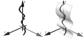
Figure 2: Left: Vessel centerline (3D curve). Right: Curved plane in 3D space.

Finding the vessel central axis can be defined as a graph theoretical problem where each voxel of the dataset is considered as a node and the transitions to the adjacent voxels as edges. Each edge is weighted by a cost function indicating the likeliness of being part of a contrast-enhanced artery. The cost function should introduce a low penalty if the edge is very likely to be within a vessel structure. Finding the path (from a user defined starting point to an endpoint) with the lowest accumulated cost within this weighted graph is known as the shortest path problem [1]. The resulting path is with high probability inside the arterial structure. Yet, the path is not necessarily the centerline of the vessel. This is, however, crucial for correct results, as deviations of the path from the central axis produce falsely simulated lesions. Therefore, the path has to be centered within the vessel before applying a curved planar reformation. First we explain the path search.

3.1.1     Cost function

The local cost function f_C(x,y) we developed for a single step from a voxel x to the adjacent voxel y can be defined as:

                                                                                   (3.1)

where a constant penalty c_step keeps the curvature of the path within the vessel low. The second component f_I(y) punishes paths tracking into regions that are beyond the intensity intervals typical for contrast enhanced arteries. In the following equations f(y) is the intensity value of the voxel y. The thresholds c_lowerBorder and c_upperBorder define the valid interval of artery density values. Within the smaller interval from c_lower to c_upper no penalty is given, as this area is regarded as optimal. With this definitions f_I(y) is:

                                                                       (3.2)

The third function f_G(x,y) results from the assumption that in the direction of the central vessel axis the gradient magnitude is lower than in the direction of the vessel boundary:

                                                                                                                   (3.3)

Finally, the fourth component f_L(y) prevents the algorithm from tracking along and into bones. A convolution with the Laplacian edge detector L is done and resulting values above a threshold c_Laplace are identified as unwanted transitions to bony structures:

                                                                                                          (3.4)

3.1.2     Implementation of the path generation

First, the user defines a starting point at the root of the vessel tree (i.e. the aorta) and an arbitrary number of endpoints marking the ends of the peripheral arteries (see figure 3a).

According to Dijkstra’s algorithm [1], all possible optimal paths to the starting point are calculated. A snap shot of this process, showing the current search space, can be seen in figure 3b. Because of the enormous size of the datasets two main performance improvements had to be done:

·      Caching temporary data: The whole dataset is subdivided into independent cache blocks. For each cache block temporary data structures as direction information and accumulated cost are allocated only if needed. Thus the memory requirements are reduced.

·      Discretizing the cost function: This method avoids the bottleneck of explicit sorting the nodes according to their accumulated cost [2]. The resulting complexity is linear to the number of voxels in the search space. Therefore, acceptable computation times can be achieved even on large datasets.

The resulting path is taken as input to a vessel center approximation algorithm as described in the following section.

3.1.3     Centering the path

For each point of the computed path a cross-sectional plane of the vessel is computed. Within this plane the true center point is calculated. The algorithm consists of four main steps:

1.    Gradient computation: This step approximates the tangent at each voxel of the original path. A B-spline curve is used in order to smoothen the gradient.

2.    Plane construction: A 2D cross section is extracted from the 3D dataset according to the current point of the original path. It’s generating vector is calculated from the B-spline curve (tangent vector).

3.    Center approximation: The true center within the 2D plane is approximated. This is done by shooting rays from the original point in the direction of the border of the vessel. Using the points at the intersections of rays and border an approximation of the center point is computed. Afterwards, the retransformation into 3D space is done.

4.    Path reconstruction: The new path consists of holes and loops because the points were moved in 3D space during step 3. These artifacts are removed using a B-spline curve again.

The centered paths can be seen in figure 3c.

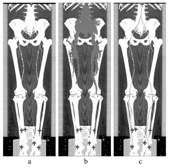
Figure 3: User-defined starting point (top) and endpoints (bottom) (a), path generation process (b) and calculated centered paths (c).

3.2     Semi-automated Segmentation

Because of the large datasets the segmentation process is kept straightforward. The user may alter the parameter settings according to the different anatomy of different parts of the body. Together with the capability of user intervention regarding the type and the spatial connection of identified objects, the method provides a useful tool for the segmentation of bones. This approach produces results, which are of diagnostical value.

The algorithm is working on so called slabs. A slab consists of several spatially adjacent volume slices. Typical 30 to 50 slices are combined in one slab. The algorithm is applied independently for each slab.

Basically the algorithm consists of 3 steps. First a rough distinction between the different objects is done. Secondly the objects are labeled. In the final step the correct shape is computed. A predefined set of parameters is used for each slab. The user can change this set of parameters during the segmentation process. For each slab the set of parameters consists of:

·        t_class: Threshold is used to distinguish different objects.

·        t_expand: Threshold to enhance already identified objects. This threshold handles partial volume effects and marrow inside the bones.

      ·       t_label: Threshold, which separates between objects considered as bones or vessels. The threshold t_label operates on the average density of objects.

First, all slices are classified using a high threshold t_class in order to distinguish different objects. The classification process is based on the intensity value and on the gradient magnitude of the voxels. The connected regions are merged and finally labeled with t_label according to their properties. The second iteration of the whole process (except of labeling) is done with a lower threshold t_expand. This step improves the quality of the segmented dataset by reducing noise caused by the partial volume effect and bone marrow. As the merging of different object types is prevented, bones and vessels remain separated. After this step a user defined labeling of objects is possible. Finally the objects labeled as bone are removed.

4.     Results

The test environment consists of a PII 350 MHz system with 704 MB main memory, running Windows NT 4.0 SR 5. The volume rendering was done on the commercial medical image processing system JVision/Space-Vision [7].

Table 1 and table 2 summarize the dataset properties and the computation times for each of the three sample datasets. Figure 4 presents the CPR of anterior tibial artery of the dataset in figure 3. Note the stent in the topmost enlargement. Figure 5 presents a comparison between the MIP of a dataset without and with a segmentation post-processing.

    

Table 1: Parameters of the test datasets.

Table 2: Investigation time of the datasets.

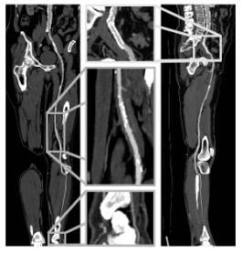
Figure 4: Coronar CPR (left side) and sagittal CPR (right side) of anterior tibial artery from the dataset in figure 3.

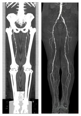
Figure 5: A MIP of a segmented dataset on the right side and a MIP of the corresponding dataset on the left side.

In figure 6 and 7 the results of the investigation methods of another dataset are shown. In contrast to iaDSA the heavy calcifications are clearly visible. Figure 7 shows non-photorealistic images done by direct volume rendering. For additional information refer to www.cg.tuwien.ac.at/~armin.

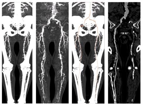
Figure 6: A sample dataset with heavy calcification. The MIP of the original dataset (left-most image) and the segmented dataset (second image) is presented in this figure. The third and the right-most image show the computed paths with a CPR corresponding to the path marked with an arrow.

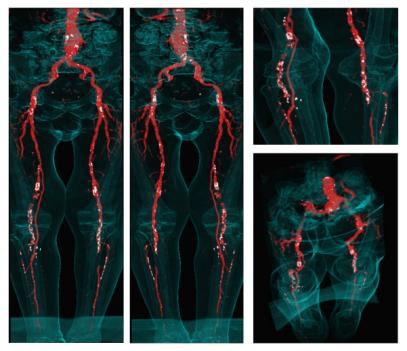
Figure 7: Non-photorealistic direct volume rendered images of the sample dataset. Calcifications and arteries are colored white and red (see also http://www.cg.tuwien.ac.at/~armin/). The outline of the body is visualized as guidance for the surgeon.

5.     Clinical Evaluation

For clinical evaluation 3 datasets from 988 to 1202 slices were post-processed manually by an experienced radiologist [4]. The same datasets were also investigated with the methods described in this work. The results were printed on laser film and a vascular radiologist compared the results vessel by vessel for lesions. iaDSA was taken as a reference standard for this purpose (see figure 8). Completely removed arteries are clearly visible errors, as whole pieces of the artery are missing. Partially removed arteries are hard to identify as errors as they look very much like stenoses. Table 3 shows that automated post-processing produces results, which are comparable to manually generated results in a much faster time.

 

Table 3: Results of the evaluation process.

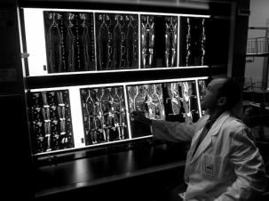
Figure 8: Evaluation of the results at the AKH-Wien.

6.     Conclusions / Future Work

We proposed in this work post-processing and visualization tools, which reduce the investigation time from 4 hours to 45 minutes. The results were of diagnostical quality and comparable to those manually generated. This could be accomplished by introducing a new cost model for vessel tracking. A tool for removing bones before visualization was implemented according to the special workflow of the diagnosis of peripheral arterial diseases.

Next steps in this project will be to enhance the reliability of the algorithms. One approach might be applying more sophisticated filter techniques [6]. Another possibility is to introduce segmentation techniques like boundary based segmentation methods in order to be able to address the non-uniform intensity values of bony structures.

7.     Acknowledgments

First of all I want to express my thanks to all people who were working on this project. Parts of this work have been done in the VRVis research center, Vienna/Austria, which is partly funded by the Austrian government research program Kplus. Other parts of the work presented in this publication have been funded by the FWF as part of project P-12811/INF (BandViz project).

8.     References

[1]   Barrett, W., and Mortensen. E., Interactive live-wire boundary extraction. Medical Image Analysis, no. 4, pp 331–341, 1997.

[2]   Falcao, A., and Udupa, J. An Ultra-Fast User-Steered Image Segmentation Paradigm: Live Wire on the Fly. IEEE Transactions on Medical Imaging, vol. 19, no. 1, 2000.

[3]   Fowkes, F., Housley, E., et. al.. Edinburgh Artery Study: prevalence of asymptomatic and symptomatic peripheral arterial disease in the general population. Int J Epidemiol, no. 20, pp. 384–392, 1991.

[4]   Kanitsar, A., Wegenkittl P., et. al.. Automated vessel detection at lower extremity multislice CTA. Oral presentation at ECR 2001, March 2 to 6, 2001.

[5]   Kanitsar, A., Advanced visualization techniques for vessel investigation. Master’s thesis, Technical University of Vienna, Institute for Computer Graphics and Algorithms, 2001.

[6]   Sato, Y., Westin, C., et. al.. Tissue Classification Based on 3D Local Intensity Structures for Volume Rendering. IEEE Transactions on Visualization and Computer Graphics, vol. 6, no. 2, pp. 160–180, April–June 2000.

[7]   TIANI Medgraph, www.tiani.com