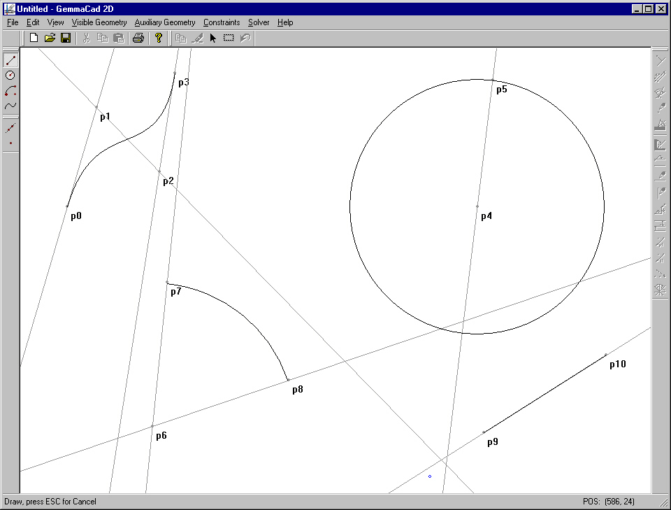
Figure 1: A Bézier curve, a circle, a circular arc, a line segment, and corresponding elements of auxiliary geometry
Franc Gerencer
Laboratory
for Geometric Modelling and Multimedia Algorithms
Institute
of Computer Science
Faculty
of Electrical Engineering and Computer Science
Maribor / Slovenia
Abstract
In the paper, some details on implementation of our new constraint-based drawing system are highlighted. The system enables users to design in a plane in an elegant declarative way by employing dependencies among geometric elements like dimensions of distances and angles, instead of calculating absolute positions. The user specifies what to draw, and not how to draw it. In the background, the constructive constraint solver is employed to establish the geometry from given relations (constraints). The main step of the algorithm is pre-processing, which first transforms various geometric elements into corresponding control points and lines only, and all types of geometric constraints into the constraints of only five different types. After this, redundant constraints of distances and angles are added, and finally, the transformed constraint problem is solved in a simple way by local propagation. A wide variety of well-constrained problems with a few exceptions can be handled, over-constrained scenes and input data contradictory to some well-known mathematical theorems are detected, and the algorithm is proved successful in many under-constrained cases as well.
Keywords: CAD, constraint-based design,
geometric constraints, geometric modelling.
1. INTRODUCTION
Conventional geometric modellers and drawing systems “think” in a procedural way. A computer program only substitutes a drawing board, but it does not offer to a designer any support by time-consuming and error-prone calculations of coordinates and dimensions. A computer is able to draw the line segment from the coordinate origin to the point (1, 1), but it does not “know” how to draw the same line segment if its length (sqrt(2)) and the slope angle (p/4) are given for example. On the contrary, a declarative description of geometry is much closer to a human. If the side lengths and the interior angles of a polygon are given, almost every one can imagine how this polygon looks like, but the computer program requires absolute coordinates of the polygon vertices, which usually does not present natural and imaginable information on object’s appearance. Therefore, the designer meets requirements for numerous additional calculations extending the design time and often presenting new sources of errors. New generation of geometric modellers offers the solution of this problem. The geometry can be described by defining relations (constraints) among particular geometric elements [1,2]. A geometric constraint is a relation among geometric objects that should be satisfied [3]. Automatic solving of geometric constraints represents some kind of an interface between a declarative description of the geometry closer to a designer, and a procedural description more suitable to a computer. This is done by a constraint solver, which presents the heart of every modern, intelligent geometric modeller. The user only specifies object’s shape and size in a declarative way, and the system takes care of making the drawing in accordance to the specification. The user specifies what to draw not how to draw it [4].
Various methods of constraint-based geometric design were presented in literature. No matter whether the constraints are employed in a plane or they operate in the 3D space, and whether they are employed on simple geometric elements only or on complex features, the methods can be classified into three main groups: the numerical approach, the symbolic approach and the constructive approach. Details can be found in [2] and [5]. In this paper, we want to emphasize importance of the constraint-based geometric design by showing applicabily of our new experimental constraint-based drawing system GemmaCAD 2D. In the system, the constructive approach to constraint solving is employed. In this approach, a pre-processing is performed to transform the constraint problem into a new form that is easy to draw. If a graph is employed for this task, so-called cycles have to be broken. The basic idea is to split the configuration into components such that each component has no cycles and all the components can be merged together in some way. Besides graphs, techniques of artificial intelligence as searching and rule-based systems can be employed in the constructive approach.
In the next chapter, the structure of the system and available user’s operations are presented. Employed geometric elements are described in the third chapter, and the constraint set is discussed in the fourth chapter. Theoretical fundamentals of the constraint solver are briefly illustrated in the next, the fifth chapter, while the reader can find more details on the algorithm in [2] and [6]. Before the conslusion, a practical example is given. Finally, our work is tried to be estimated, original contributions are stressed once more, and some details intended to be improved and implemented in the future, and some problems still waiting to be solved are emphasized.
2. GemmaCAD 2D
The presented system named GemmaCAD 2D operates in 2D space. The majority of constraint types and some other features like division of geometry into the visible and auxiliary part were inherited from two constraint-based drawing systems, implemented by our group in the past – FLEXI and BFoFD (see [1] and [7]). But these two systems suffered from several disadvantages intended to be abolished with the new system:
In BFoFD [7], points, lines, line segments, circles, circular arcs, ellipses, Bézier curves, and rather rich constraint set were employed, but the constraint solver was not powerfull enough to handle successfully all geometric problems that could have been described by the user. GemmaCAD 2D was developed to fill this gap between theory and practise.
The work with GemmaCAD 2D is performed in a similar way as with BFoFD or any other constrant-based drawing system. A user can perform the following actions:
3. GEOMETRIC ELEMENTS
3.1. Visible and Auxiliary Geometry
GemmaCAD 2D employs a two-level organisation of geometric objects that was introduced with BFoFD [7] already. Bézier curves, circles, circular arcs, and line segments form the visible geometry, and they are mapped onto control points and lines forming the auxiliary geometry. Each entity of the visible geometry has its equivalent (or more of them) in the auxiliary part, and the opposite is not necessary. In Figure 1, we can see examples of all mentioned types of the visible geometry and their underlying auxiliary geometry.
Figure 1: A Bézier curve, a circle, a circular arc, a line segment, and corresponding elements of auxiliary geometry
The two-level organisation is important because of the following facts:
Geometric elements can be added interactively by a mouse or through a dialog box. If the data entered in a dialog box are not complete, then we complete it in a graphical editor by the mouse. In the graphical mode, we can see intermediate results.
Let us discuss posibilities how a line segment can be added. When we are moving the mouse, the mouse cursor presents the first end-point of the line segment. By pressing the mouse button, the position of this point is selected. During forder mouse moving, an intermediate line segment between the previously selected end-point and current cursor position is drawn. By pressing the mouse button again, the cursor position is selected for the second end-point, and the line segment is drawn in style presenting the visible geometry. A new node in the list of line segments, two nodes in the list of points, and a node in the list of lines are created. Coordinates of both end-points are written into the point nodes, and the line slope is witten into the line node. The line segment node contains pointers to all three nodes of the auxiliary geometry.
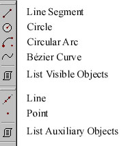
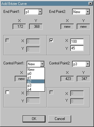
When a geometric element is added through a dialog box, there are more possibilities. We can choose auxiliary points from the list, or we can insert absolute coordinates in corresponding edit boxes. If this last possibility is employed, the Point constraint is automatically added, and the point position is fixed. Such point cannot be moved later when the constraint solving is performed. All the control points describing an element of the visible geometry need not be selected in the dialog box already. After leaving the dialog box, the system requires their insertion in the graphical mode. In Figure 2, we can see the toolbox for selecting a type of geometric elements, which are intended to be inserted or selected in the graphical mode. In Figure 3, the dialog box for adding or editing a Bézier curve is shown.
Figure 2: Toolbar for geometry types Figure 3: Adding a Bézier curve through the dialog box
If we want to delete or edit a geometric element, it has to be selected first. This can be done in the list of geometric elements of the appropriate type or in the graphical mode. We can select a single object or we can capture all objects inside some interactively entered rectangular area in the graphical editor. When an object of the visible geometry is being deleted, the underlying elements of the auxiliary geometry have to be deleted, too. For this reason, the data structure presenting an element of the auxiliary geometry contains a pointer to the owner i.e. an object, which has created this element. Automatically created constraints also have owners. When an element of the auxiliary geometry is deleted, all constraints refering to it are also deleted.
When a geometric element is edited, the same dialog, which is used for adding the elements of the corresponding type, is employed. But only the element's numerical attributes can be modified in this dialog. Pointers to underlying elements of the auxiliary geometry may not be changed.
4. GEOMETRIC CONSTRAINTS
The constraint employed in GemmaCAD 2D operate on elements of the auxiliary geometry i.e. points and lines only. They can be classified into four groups:
4.1. The Constraint Set
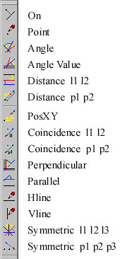
In the current version of the program, fifteen constraint types are implemented. There are a topological constraint On(p, l) that requires that the point p lies on the line l, eight dimensional constraints Distance(p1, p2, d), Angle(l1, l2, a ), Parallel(l1, l2), Perpendicular(l1, l2), RelPos(p1, p2, x, y), Coincidence(p1, p2), Coincidence(l1, l2) and Distance(l1, l2, d), four positioning constraints Point(p, x, y), AngleValue(l, a ), HLine(l) and VLine(l), and two structural constraints Symmetric(p1, p2, p3) and Symmetric(l1, l2, l3). We have also developped the whole theory about structural constraints establishing sums and ratios of distances or angles, and therefore, at least ten new constraint types will be available in the next version.
4.2. Original and Transformed Constraints
With the declarative description of geometry, we meet an important problem: it is much easier to define constraints than to solve them. Our constraint set enables a user to describe a constraint problem in an elegant way, but particular constraints are much too complex to be solved directly by local propagation. The problem is solved by replacing these constraints by sets of simpler ones. We need only the constraint types to define the following relations: distance between two points – Distance(p1, p2, d), angle between two lines – Angle(l1, l2, a ), absolute position of a point – Point(p, x, y), absolute slope of a line – AngleValue(l, a ), and the topological constraint On(p, l). Each constraint of the original constraint set C is therefore defined as a conjunction of the predicates mentioned above. The transformed constraint set is named the minimal constraint set Cmin. The constraints from Cmin are explicitely defined constraints, and the constraints from the original set C are original or user-defined constraints. Some original constraints cannot be presented by employing predicates from Cmin on existing elements of the auxiliary geometry only. They require additional points and lines to establish some relations, but a user need not be aware of their existence. These points and lines present so-called invisible geometry.
Two-level constraint organisation results in the following advantages:
A user can only add, insert or edit original constraints. When he wants to add a constraint, he has to select the constraint type first. This can be done in the constraint toolbar (see Figure 4) or in the main menu. After this, geometric elements (points and lines) envolved in the relation presented by the constraint have to be selected. Selection is done in the graphical mode or from the object list activated from a dialog box. Numerical parameters can be entered in the dialog box only.
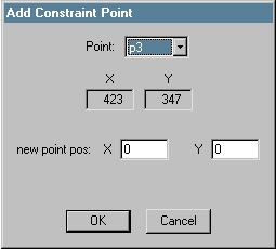
Figure 4: The Constraint Toolbar Figure 5: Add Point from dialog box
When a constraint is being deleted, the underlying transformed constraints and invisible geometry are also deleted. When a constraint is edited, only numerical parameters may be modified.
5. THE ALGORITHM
The whole theory about the constraint solver employed in GemmaCAD 2D can be found in [2] and [6]. Only the most important things will be repeated here. The algorithm works in several steps, which can be grouped into three main parts: pre-processing, constraint solving, and final preparing of the results.
The main phase is the pre-processing, which transforms a constraint problem into a form that is easy to be solved. The first two steps of this pre-processing were discussed already: mapping the visible geometry onto the auxiliary geometry, and decomposition of complex original constraints into the transformed constraint set consisting of constraints of only five different types.
The last step of pre-processing is the most complex part of the algorithm. First, it introduces two matrices: the matrix of distances MD and the matrix of angles MA. They are filled by numerical attributes of predicates Distance and Angle from Cmin, or by dimensions from the drawing in the case that an explicitely defined constraint does not exist. Matrix elements filled by attributes of explicitely defined constraints may not be changed any more, and therefore they get higher priority than elements initialised from the drawing. The matrices are then employed for solving the triangles and determining the sums and the differences of angles sharing common edges. These operations modify values and raise prioritieres of particular elements of both matrices. The goal is to fill the matrices as much as possible. The matrix is full if it does not contain elements with the low priority any more. This step can be understood as adding redundant dimensional constraints of distances and angles. The redundant constraints play an important role because they can be employed to determine other values in both matrices, and they can be chosen for constraint solving instead of explicitly defined constraints. In this way, cycles can be avoided.
All that we need for constraint solving are sets of lines L and points P containing the elements of the auxiliary and invisible geometry, the matrices MA and MD, and the predicates On, Point and AngleValue from Cmin. The algorithm splits the sets L and P into the components named clusters, solvable with local propagation. Each cluster contains lines with known mutual angles and all the points lying on these lines. When the matrix of angles MA is full, we obtain a single cluster. This happens with the majority of well constrained problems, and with some under-constrained problems as well. Over-constrained problems were detected in the previous step of filling the matrices as well.
Predicates On, Distance (obtained from MD) and Angle (MA) in particular cluster are solved in a simple way by local propagation. After this, clusters are merged together by solving predicates Distance connecting points of different clusters. The last step of the algorithm solves eventual positioning predicates AngleValue and Point. The constraint decomposition into the transformed constraint set ensures that no more than one predicate Point and also at most one predicate AngleValue are present in Cmin. The predicate AngleValue requires rotation of the whole scene around the origin, and the predicate Point is satisfied by translation of the desired point into the required position, and then translation of all other points and lines for the same offset (for more details, see [2] and [6]).
Auxiliary geometry is positioned after the step of constraint solving, and all that is left is to establish the visible geometry from it.
6. RESULTS
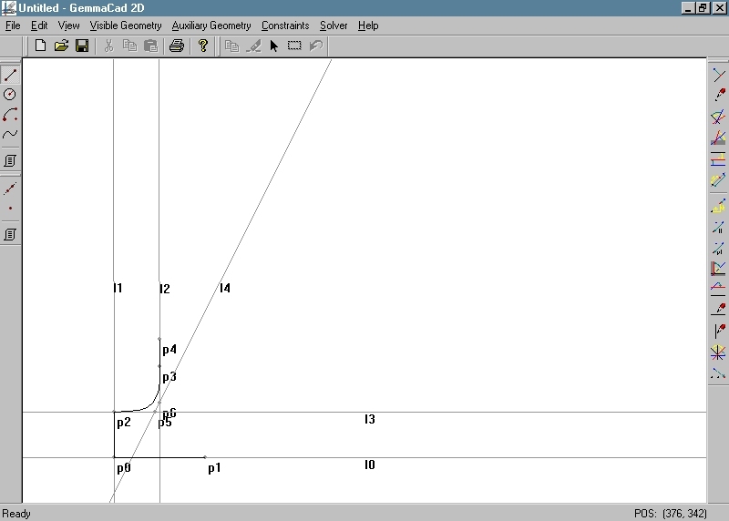
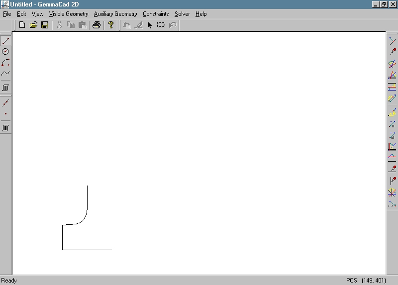
Let us conclude this paper with a practical example of drawing with GemmaCAD 2D. One of possible applications of the program is intelligent font design. That was also the reason why BFoFD (Basic Font Feature Designer), the predecessor of GemmaCAD 2D, was developed years ago [7]. Let suppose the user wants to draw a part of the Times New Roman letter “I”. The letter can be seen as a union of four symmetric parts. It suffices to establish the topology of all these four parts, to determine geometry of one of them by employing dimensional constraints, and then to employ structural predicates Symmetric to detail other three parts. The initial sketch presenting the bottom left quarter of the letter is shown in Figure 6. In Figure 7, the auxiliary geometry is also visible.

Figure 6: Initial sketch of left bottom quarter of “I”
Figure 7: Visible and Auxiliary Geometry in the initial drawing
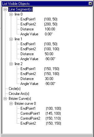
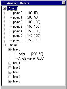
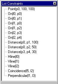
Figure 8: Visible geometry, auxiliary geometry and original constraints presenting the detailed left bottom quarter of “I”
Figure 9: Constrained quarter of “I”– Visible and Auxiliary Geometry
Figure 10: Constrained quarter of “I” – Visible Geometry
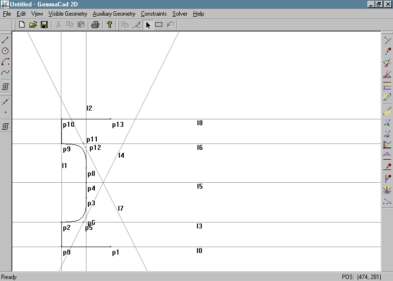
Figure 11: Left half of the letter “I” – Visible and Auxiliary Geometry
In the paper, we have described how our new constraint-based drawing system GemmaCAD 2D can be employed for intelligent geometric design. The system enables users to design in a plane in an elegant declarative way by employing relations (constraints) among geometric elements like dimensions of distances and angles, instead of calculating absolute positions. The user specifies what to draw, and not how to draw it. GemmaCAD 2D was developed to solve some problems met with our previous system BFoFD [7]. The main disadvantages of that system were that it was not incremental at all, and also not variational. Beside to this, it failed to find a solution in the majority of cases containing cycles. We believe that our new system is much more successfull and efficient. The heart of the system is a constructive constraint solver which operates in three phases. The main step of the algorithm is pre-processing, which first transforms various geometric elements into corresponding control points and lines only, and all types of geometric constraints into the constraints of only five different types. After this, redundant constraints of distances and angles are added, and finally, the transformed constraint problem is solved in a simple way by local propagation. We believe that particular steps, specially the pre-processing present original and efficient contributions of our group in the field of geometric constraint solving.
ACKNOWLEDGEMENTS
I would like to thank to David Podgorelec, MSc, from the Faculty of
EE & CS of the University of Maribor, the author of the theoretical
fundamentals of this project, for his suggestions and advices during the
system implementation and preparing this paper.
| [1] | Žalik,B, Guid,N, Clapworthy,G: Constraint-based Object Modelling. Journal of Engineering Design Vol.7, No.2, pp.209–232, 1996. |
| [2] | Podgorelec,D, Žalik,B: A geometric constraint solver with decomposable constraint set, Skala,V (ed.) The 9th International Conference in Central Europe on Computer Graphics and Visualisation’01 - WSCG’01, Plzen, Czech Republic, University of West Bohemia, Vol. 2, pp. 222–229, 2001. |
| [3] | Freeman–Benson,BN, Maloney,J, Borning,A: An Incremental Constraint Solver. Communications of the ACM, Vol.33, No.1, pp.54–63, 1990. |
| [4] | Sunde,G: A CAD System with Declarative Specification of Shape, Eurographics workshop on Intelligent CAD Systems, Noordwijkerhout, The Nederlands, 1987. |
| [5] | Gao,X–S, Chou,S–C: Solving geometric constraint systems. I. A global propagation approach, Computer-Aided Design, Vol.30, No.1, pp.47–54, 1998. |
| [6] | Podgorelec,D: Approaches to solving cycles in constraint-based geometric design, Master Thesis, University of Maribor, Faculty of EE & CS, Maribor, Slovenia, 2000 (in Slovene language only). |
| [7] | Kolmanič, S., B. Žalik, “Interactive Variation of Geometric Shapes Inside a Constraint Based Environment”, in N. M. Thalmann and V. Skala (Eds.) The Fifth International Conference in Central Europe on Computer Graphics and Visualisation’97 - WSCG’97, Plzen, Czech Republic, 1997, Vol. 1, pp. 222–231. |
| [8] | Bouma,W, Fudos,I, Hoffmann,C, Cai,J, Paige,R: Geometric Constraint Solver, Computer Aided Design, Vol.27, No.6, pp.487–501, 1995. |
| [9] | Fudos,I, Hoffmann,CM: A Graph-constructive Approach to Solving Systems of Geometric Constraints, ACM Transactions on Graphics, Vol.16, No.2, pp.179–216, 1997. |