Geometry compression and multiresolution

Multiresolution compression and feature
line reconstruction for Reverse Engineering

Giuseppe Patané, Corrado Pizzi, Michela Spagnuolo

{patane, corrado, spagnuolo}@ima.ge.cnr.it

Istituto per la Matematica Applicata

Consiglio Nazionale delle Ricerche,

Via De Marini 6,

Genova 16149, Italy

1 Abstract

In this paper we analyze applications of Douglas-Peucker algorithm to compression and feature line extraction of 3D models from digital scans introducing a multiresolution model that enables a fast description of the object at different levels of details through the use of a unique rearrangement, stored in a file, of the input data set. The multiresolution algorithm, which reaches high data compression rates while producing fair approximation, is used to simplify each point of the input data set according to its scale, its basic shape type and its geometric parameters. Finally, object feature lines are reconstructed using shape information previously found. The proposed algorithm is able to segment the object into meaningful patches, which represent form features of the object, resulting in an important tool for reverse engineering and rapid prototyping.

KEYWORDS: Compression, Multiresolution Analysis, Feature Lines, Reverse Engineering, Rapid Prototyping, Douglas-Peucker algorithm.

2 Introduction

While in the traditional approach, objects are manufactured starting from a CAD model in reverse engineering real parts or object prototypes are transformed into CAD-like models that can be modified with different mathematical transformations providing a great flexibility to the design phase. The process of CAD model starts from a set of points, which are acquired on an existing object with several methods such as tactile or non-contact ones. The resulting data set, unorganized (laser scanners) or partially ordered (digitizing machines), is transformed into polyhedral or smooth surface converting therefore its discrete description into a piecewise, continuous model.

A basic step towards the creation of a CAD-like model, is the so-called segmentation. Its aim is the logical subdivision of the input, generically a set of points, in subsets such that each of them contains points belonging only to a specific surface type [2]. The approaches used for the segmentation process are general or dedicated [3]. The first ones use only general knowledge of surfaces to execute the segmentation, while the dedicated approaches, that are preferable, search for particular structures in the data set [3]. Furthermore, the connectivities and continuity in the data structure of the model is very important and a low-level description, such as a simple collection of faces in not enough [2] and a decomposition into functional patches would be desirable in the majority of CAD/CAM applications.

In this sense, the work presented in this paper is concerned with the definition of high-level polyhedral models of the object skin, which is eventually described as a set of feature lines [4]. Starting from this model, we are seeking to segment the surface into machining meaningful patches representing form features of the object.
Out approach to set up a high level description of a data set is described in the following steps:

level of detail simplification: compression through a multiresolution analysis. This phase aims at reducing sampled points to a minimal number discarding the ones which do not locate important shape elements. Therefore the main goal of simplification is to generate a low approximation that maintains the main features and overall appearance. The number of sampled points necessary to represent a data set accurately depends on the model and on its characteristics with respect to its morphological structure,
scan line analysis: shape feature classification using a scale-base and geometric characterization of features that allows to distinguish local and global details,
feature lines detection: extraction of feature lines or curves achieved joining points which lie on adjacent scansion lines judged similar according to the measures defined in § 5.

The paper is organized as follows. First data compression and simplification technique are presented. Then the measures used to classify the shape feature of the scansion lines are introduced and, finally, the determination of the feature lines and considerations about the segmentation process are given.

3 Data compression

New scansion technologies have accelerated, on the one hand, the manufacturing process providing dense data set in order to achieve accurate reconstructed products and have brought, on the other hand, the need of discarding redundant information. The aims of data compression [2,3,5,10,16] is to preserve the shape and to control locally the approximation error. Its main advantages are a large decrease of storage requirements, a lower cost for visualization and a fast transmission, which is important for web-based applications where bandwidth limitation becomes a major concern. Furthermore, this step also represents a preprocessing with respect to classification of shape features.

In the choice of data compression algorithms for reverse engineering, the constraint is the no-repositioning of sampled points, that is, the compressed data set has to be a subset of the original one.

First of all, the sampled object is assumed to be a 2.5D surface with points distributed on parallel planes that define a sequence of scansion lines.

Definition. Let be F: = { (x,y,z) ‘R³:f(x,y) = z } a single-valued function defining the object surface, and S: = { (x,y,z) ‘ R³: ax+by+c = 0 } a plane. A scansion line L is an ordered sequence of (n+1) points L: = { P₀(x₀,y₀,f(x₀,y₀)),..., P_n(x_n,y_n,f(x_n,y_n)) } such that L is common to F and S and at least one between (x₀,...,x_n) and (y₀, ..., y_n) is a closely increasing or closely decreasing sequence. Then, the sampling of F with respect to the scansion direction defined by the normal vector (a,b,1) to a set of planes S_i = {(x,y,z) ‘ R³:ax+by+c_i = 0} i = 0, º,k is represented by L₀, ...,L_k where each L_i is the scansion line on F with respect to S_i with c_i > c_i+1.

Given a 3D-set P = {P_i}_{i = 0}ⁿ, associated with the polygonal curve S(P₀,º, P_n) obtained connecting consecutive points P_i,P_i+1, i = 0, º, n-1 with a line segment, we want to define a new set Q = {Q_i}_{i = 0}^m such that

Q is a subset of P (m £ n),
the error between the data points and the fitted line is less than a maximum tolerance with respect to the Hausdorff distance d defined by the following relation

d(X,Y): =

max

{d_X(Y), d_Y(X)}

d_X(Y): =

sup
y ‘ Y

{

inf
x ‘ X

{||x-y||₂}}

₂

Suppose we are given a chain with n segments, the Douglas-Peucker hierarchical algorithm [3,16] sorts points {P_i}_{i = 0}ⁿ in decreasing order of importance with respect to the criterion that will be defined using the distance d. Therefore we have to settle the permutation j: {0, ..., n} ---> {0, ..., n} that represents the rearrangement of the input data set.

The first step selects endpoints of the line segment S(P₀,º, P_n) choosing j(0) = 0 and j(1) = n. Constructed S(P_j(0), P_j(n)), which combines P₀ to P_n, the algorithm picks out the point P^* that satisfies the relation

d(P^*, S(P₀, P_n)) =

max
i = 1, º,n-1

{d(P_i,S(P₀,P_n)}.

If P^* = P_k we update j choosing j(2) = k and we split the chain at this vertex obtaining two new polylines (P₀P_k) and (P_kP_n). In every subset of the input line the splitting point, which is the farthest vertex from the line segment that joins local endpoints (i.e local anchor and floater), is recursively selected and the index of the point with maximum distance gives the value of j for the step in issue. After at most (n-1) steps, points will be hierarchically reordered.

The method provides a sequence (P_j(i), d_i^H)_{i
= 0}ⁿ that is used for the description of the object at different levels of details: for instance, to find the polygonal chain that satisfies the relation

d(S(P₀, º, P_n), S(Q₀, º, Q_m)) £e

(1)

the choice is to set {Q_i = P_j(i)}_{i = 0}^m with m such that

d_i^H „e i = 0, º, m, and d_m+1^H < e

where the reduction percentage (100*[(n-m+1)/( n+1)]) % depends on the setup tolerance.

The common use of this simplification method has a different approach to reduce the number of points of a dense sampled data set with the use of a tolerance band e. At a given step we approximate the chain from P_i to P_j with

the line segment (P_iP_j) if the farthest vertex P^* from this segment has distance at most e, otherwise
we will split the chain at this vertex applying the criterion recursively to the new polylines (P_iP^*) and (P^*P_j).

We observe that the output of the algorithm is equal to the previous subset of P but it has been preferred to stop the calculation after (m+1) steps constructing the set of indexes {j(0), ..., j(m)}. Therefore the upper bound of the evaluation of the distance formula, which is the most time consuming part of the procedure, is O(mn) rather than (nlog₂n) required for a total rearrangement of the data set [6].

We can modify the previous situation such that will be demanded in input to set up a data reduction rate rather than a tolerance band. This choice is justified by a greater simplicity that it finds commonly in estimating this parameter regarding the choice of the maximum approximation error e. Set up a value k we consider the set {Q_i = P_j(i)}_{i
= 0}^m with m: = [[(100-k)/ 100] ×(n+1)] where [ ] is the integral part. This choice allows to obtain the polyline S(Q₀, ...,Q_m) which fulfills (1) with e = min_{i = 1, ...,m}{d_Hⁱ} and the result is achieved writing in an ASCII file, for every polyline, the rearrangement represented by the permutation j and its array of distances (d_Hⁱ)_{i
= 0}ⁿ (d_H⁰ = d_Hⁿ = 0). To summarize, our approach to compression allows to reduce the time needed to switch from a level of detail to another, without additional cost: indeed only the simple reading of the indexes j(i), which characterize the points of the output, is required without any distance computation.

4 Multiresolution analysis and simplification

In this section, we want to define the multiresolution approach to the description of a sampled data set through the Douglas-Peucker. Consider a set of points in R³, expressed as a column vector of sampled points S_n: = [P₀, P₁, ...,P_n]^T. We wish to construct a low resolution version S_n-1 of S_n with a fewer number of points m. The standard approach [2] to its construction is represented by a (m, n+1) matrix such that the relation S_n-1 = A_n*S_n holds. In the filtering process from S_n to S_n-1 (n-m+1) points will be omitted with an amount of detail lost that will be estimated regarding the Hausdorff distance d. We indicate therefore with D_n-1 the lost detail of S_n through the relation D_n-1 = B_n*S_n with B_n (n-m+1, n+1) matrix and we refer to A_n and B_n with the term of analysis filters while the splitting of S_n in (S_n-1, D_n-1) is called decomposition. Applying recursively this method we are able to express the initial set of points through a hierarchical structure of low resolution descriptions S₀,..., S_n-1 and of details D₀, º, D_n-1. This process, called filter bank, is summarized in (2).
Since S_n, as we will see in the following pages, can be reconstructed from the sequence S₀, D₀, ..., D_n-1 the filter bank represents a hierarchical transformation of the sampled data set.

Introduced the outline base for the multiresolution analysis we have to specify:

the criterion of construction of A_k and B_k "k = 1, ..., n-1,
the error achieved in the compression process from S_n to a lower resolution S_k,
the expression of S_n through S₀, D₀,..., D_n-1.

To this end we consider a decreasing sequence of real non-negative tolerance bands that belong to the a-set {d₁, º,d_n: d₁ > ... > d_n, n „ 1 } and we define with

S_k the data set achieved applying to S_k+1 the Douglas-Peucker algorithm with tolerance band d_k+1 "k = 0, º, n-1,
D_k: = S_k+1-S_k "k = 0, º, n-1 the data set of detail,

Each element of the a-set represents the width of a tolerance band and the simplification error d_n. From previous relations we have that S_k Õ S_k+1 and we can construct the sequence and its filter bank with

S_k = {P_j(i) ‘ S_k+1: d_Hⁱ „>= d_k+1} = {P_j(i) ‘ S_n:d_Hⁱ„>=d_k+1 }

and

D_k = {P_j(i) ‘ S_n: d_Hⁱ ‘ [d_k+2, d_k+1) }.

We conclude that S_k-1 is achieved applying the algorithm with band d_k+1 either to S_n or to S_k.

Therefore the original data set is uniquely decomposed using the low resolution description S₀ and the detail sets (D_k)_{k
= 0}^n-1. Finally, the evaluation of the error carried out in the compression process from S_i to S_k (i > k) is

d(S_i,S_k) £ d_k+1.

The accuracy of the process has to be tuned on the width of the value d_n and all lines have to be simplified using a unique a-set of tolerance bands. Problems may arise in the choice of this set due to unbalanced density and dimension of feature shape (a possible way to solve this problem is re-calibration of the a-set). In shape line analysis tolerance bands are defined using the following relation

d_i: = i ×

d₁n

i = 1, ..., n

with d₁ maximum global error (i.e maximum error of every polyline).

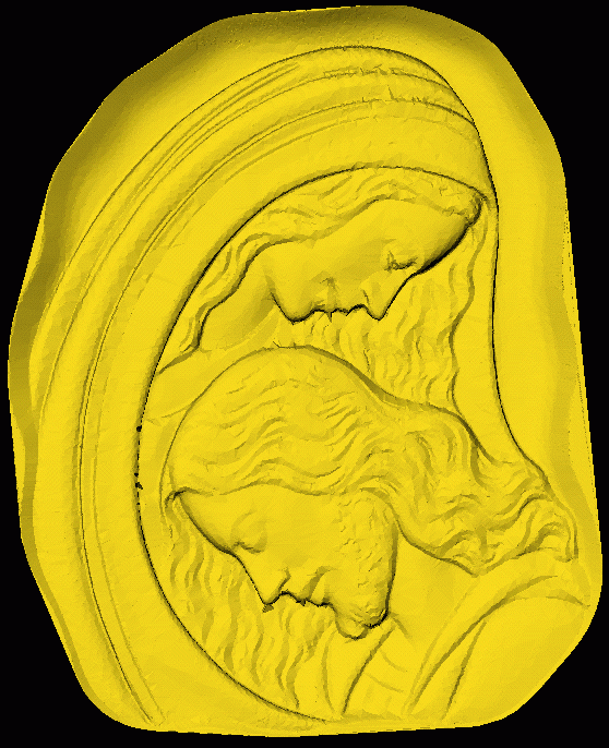
Figure 1: Original data set with 1.328.531 points structured in 1.214 polylines

Figure 2: Result of compression: compressed data set with 66.427 points, date reduction 95% .

5 Scansion line analysis and feature line detection

The aim of scansion line analysis, which relies on the assumption that the shape of next scansion are similar for densely defined data set, is a classification of shape features and it represents the background for shape reconstruction. Therefore feature lines of the object will be locally compound of similar points with respect to shape similarity defined in the following.

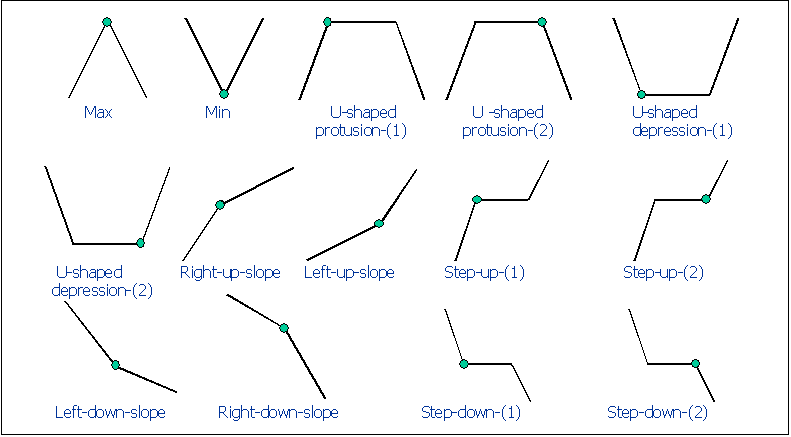
As described in the previous section the Douglas-Peucker method, with a user defined a-set, enables to obtain a first description of points of a scansion line with respect to size of shape features. Beside this scale analysis, which codes sizes of features, we consider geometric parameters with the aim to classify their type. The adopted scheme (see tab.1), which uses three points to describe a feature, identifies shapes meaningful for producing a decomposition relevant with respect to traditional basic approach in CAD contexts.

Figure 3: Tab. 1 Mathematical description of the primitive shape elements. For each configuration, squares represent points where the label will be added

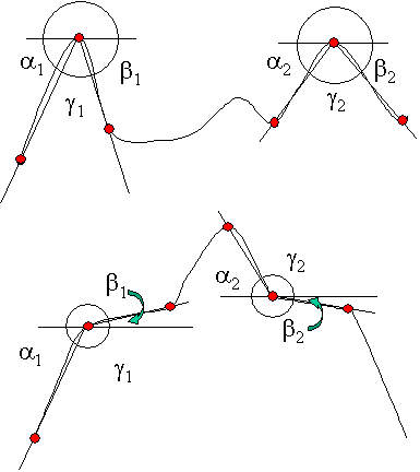
The second classification (see tab.2), based on angular measures d, b that are introduced regarding the same triplet of points according to the previous classification, distinguishes among shape features evaluating their amplitude and orientation.

Using the a-set, the previous classification and the angular measures we are able to introduce three basic similarity "relations" on the input data set:

a-width similarity: P ‘ L_P, Q ‘ L_Q

P ~ _a Q <---> width(P) = width(Q)

feature similarity: P ‘ L_P, Q ‘ L_Q

P ~ _T Q¤ <---> T(P) = T(Q)

geometry similarity: P ‘ L_P, Q ‘ L_Q

P ~ _GQ <---> their orientation and inner angles are similar

Beside shape characterization, the suggested measures are used, on the one hand, for evaluating similarity among shape features and, on the other hand, for reconstruction of the last ones. This method recognizes feature lines in directions almost orthogonal to the scansion one by linking similar points from a line to a next one. Using the previous relations, two points P, Q ‘ R³ will be connected if and only if

P ~ _a Q, P ~ _TQ, P ~ _G Q.

Moreover, distance among points is considered with the purpose of maintaining fidelity of line recognition that decreases increasing the first one. Following the approach in [15] an influence cone, with a variable axis oriented in the direction of the lines to reconstruct, is used to select portion of adjacent line relevant for reconstruction. We underline that a crucial part of the algorithm for detection of feature lines is the selection of the part of similar points, because there may be a considerable number of candidate points as well as none. Furthermore, scanning direction is fundamental because feature lines whose directions are almost parallel to it will be, generally, impossible to detect with this approach.

Figure 4: Tab. 2 Classification of feature based on angular measures.

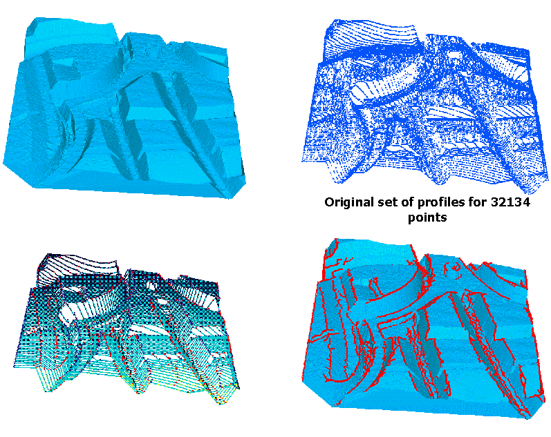
Figure 5: Application of the method to a 2.5D example.

6 Conclusion and further works

The proposed method introduces the multiresolution analysis and shape feature detection of a highly detailed and densely defined data set with the use of a unique rearrangement, stored in a file, of the input which enables a fast description of the object at different levels of details. Furthermore, any level of detail can be accessed directly maintaining geometric behavior according to the needs of the problem domain where a rough approximation S₀ is superseded by subsequent refinements. The algorithm reaches therefore high data reduction rates while producing fair approximations.
Our strategy to subdivide a surface in shape features, is based on the consideration that a scansion line is a section of the surface and this imply that the first one contains sections of the shape features of the surface. The segmentation, that is the classification of each point as belonging to a specific feature class, will be driven by the feature lines detection. The method that we are developing considers simple and compound of features in the surface, which can be detected thanks to multiscale approach That provides a hierarchy among points features.

7 Acknowledgements

The authors would like to thank the Technimold S.r.l, Genova-Italy, for the fruitfull cooperation during the Project "Sviluppo di tecnologie innovative per il Reverse Engineering e il Rapid Prototyping ed analisi comparative" ¹ and for the data provided for this work. Special thanks are given to Dr. Bianca Falcidieno, IMA-CNR, for the valuable help and support.

References

[1]: Buttenfield, B.P.: A rule for describing line feature geometry. In: B.P. Buttenfield R. McMaster (eds) Map generalization, Chapter 3, (1997), 150-171.
[2]: DeRose, T., Salesin D. H., Stollnitz, E. J.: Wavelets for Computer Graphics: A primer, part 1. IEEE Computer Graphics and Application, 15(3): 76-84, May 1995.
[3]: Douglas, D.M., Peucker, T.K.: Algorithms for the reduction of the number of points required to represent a digitized line or its caricature. The Canadian Cartographer, 10/2, 1973, 112-122.
[4]: Falcidieno, B., Spagnuolo, M.: Shape abstraction tools for modeling complex objects. Proocedings of the international conference on shape modeling and applications, 1997, IEEE Computer Society Press, Los Alamos, CA.
[5]: Fisher, A.: A multi-level for reverse engineering and rapid prototyping in remote CAD systems. Computer Aided Design 32 (2000), 27-38.
[6]: Hershberger, V., Snoeyink, J.: Speeding up the Douglas Peucker line simplification algorithm. Proc. 5th Intl. Symp. on Spatial Data Handling, Vol.1, Charleston, SC, (1992), 134-143.
[7]: Hoffman, D., Richards, W.: Representing smooth plane curves for visual recognition. Proc. of American Association for Artificial Intelligence, Cambridge, MA: MIT Press (1982), 5-8.
[8]: Hoschek, J., Dietz, U., Wilke, W.: A geometric concept of reverse engineering of shape: approximation and feature lines. In: M. Daehlen, Lynche T. and Schumaker LL. (eds): Mathematical methods for curves and surfaces II, Vanderbilt University Press,(1998) Nashville.
[9]: R. McMaster. A statistical analysis of mathematical measures for linear simplification. The American Cartographer 13, 2 (1986), 103-117.
[10]: Patané, G.: Metodi di compressione e analisi multirisolutiva per il Reverse Engineering. Rapporto di attivitá-Istituto Nazionale di Alta Matematica "F. Severi"( Scuola per le Applicazioni della Matematica nell' Industria)- Universitá Degli Studi di Milano, Polo Bicocca, Dipartimento di Matematica e Applicazioni.
[11]: Patrikalakis, N. M., Fortier, P.J., Ioannidis, Y., Nikdaon, C.N , Robinson, A. R., Rossignac, J. R., Vinacua, A., Abrams, S. L.: Distributed Information and Computation in Scientific and Engineering Enviroments. M.I.T 1998.
[12]: Plazanet, C.: Measurements, characterisation and classification for automated linear features generalisation. Proceedings of AutoCarto 12, 4, Charlotte CA:ASPRS and ACSM, 1995.
[13]: Plazanet, C.: Modelling Geometry for Linear Feature Generalization. In: M. Craglia, H. Coucleis (eds), Bridging the Atlantic, Taylor & Francis (1997), 264-279.
[14]: Plazanet, C., Spagnuolo, M.: Seafloor Valley Shape Modelling. Proc. of Spatial Data Handling , Vancouver, (1998).
[15]: Spagnuolo, M.: Shape-based Reconstruction of Natural Surfaces: an Application to the Antarctic Sea-Floor. In M. Craglia, H. Coucleis (eds), Bridging the Antarctic, Taylor & Francis (1997).
[16]: Saux, E.: Lissage de courbes pur des B-splines, application á la compression et á la généralisation cartographique. PhD Thesis, Nantes University, France, January 1999.
[17]: Varaday, T., Martin, R., Cox, J.: Reverse engineering of geometric models, an introduction. Computer Aided Design, Vol. 29, No. 4, (1997), 255-268.

Footnotes:

¹ Progetto nato dall' azione finanziata dalla Regione Liguria nell' ambito del settore Politiche di Sviluppo Industria e Artigianato, DOCUP Ob. 2 (1997-1999) - Az 4.2 Sviluppo dell' innovazione di cui è titolare Technimold S.r.l.

File translated from T_EX by T_TH, version 2.25.
On 22 Mar 2001, 17:58.