Pattern recognition using genetic algorithms

Juro Gottweis,

juro@email.com

Faculty of Mathematics, Physics and Informatics
Comenius University
Bratislava / Slovakia

Abstract

This paper describes one possible approach to the pattern recognition problem. The described approach is inspired by current knowledge about visual pathway in animals.

The main idea behind the described approach is to use genetic algorithms to create small structured programs. These programs are subject to test of their ability to recognize a given pattern. They are improved by continuous process of selection, crossover and mutations.

Tests as well as observations are part of this paper. Early processing of visual information in animals is also briefly described.

Keywords: pattern recognition, genetic algorithms, vision.

1. Introduction

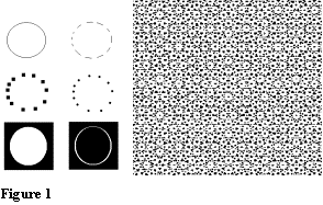
Let’s look at Figure 1. Why do we see circles on the pictures? How does our brain recognize these circles? These were some of the questions that inspired me to work on this paper. One possible method to answer these questions is to study and to try to understand brain. We can call it a top-down approach. Although it is surely very interesting, I’ve chosen a different method. In this bottom-up approach I am trying to build structure that is able to recognize patterns. This structure utilizes some of the known principles from visual recognition in animals. I hope that parallels between this created structure and visual pathway will allow us to better understand the principles how our brain works and to answer the questions mentioned above. However we should say at the beginning that although we have some preliminary results, this work is far from giving final answers.

2. Overview

Patterns are recognized by small structured programs. These programs (I will refer to them as creatures) are evolved in groups called populations. The genetic algorithm creates the population, tests its members, then based on the results of testing creates new population etc. The number of creatures in the populations is constant. A creature in a new population is created by the combination of the codes of two creatures from the current population. Creatures that have been better in pattern recognition have a better chance to have an offspring (more on this subject in section 6: The inputs). The implemented algorithm supports evolution of more than one population. These populations evolve almost independently; just time-to-time they exchange their best members. More about this is written in section 7: Testing and the observations. This paper contains short introduction to the visual recognition in animals. Reader who is familiar with the issue should jump directly to section Creature’s structure.

3. Vision in animals

This chapter describes knowledge about animal’s visual center related to my work. I think that after reading it, it will be clearer why I have chosen the specific structure for creatures as well as the specific features in the proposed language. Similarly to Fukushima’s neocognitron [5], I have based the architecture on the principles described in this chapter.

Visual information is processed by the layers of cells. A layer sends processed information to other layer or layers. Thus we can say that vision in animals is hierarchical. Another interesting feature of the cells (at least at the first partially explored stages of visual recognition) is that we can describe cell functions in regular sentences like: “ganglion cells in the retina work as detectors of contours in the image.” or “simple cells in primary visual cortex are detecting small lines with specific orientation”. That means that to understand the cells we don’t need to describe the settings on the cells synapses and other attributes. We can formulate their task (to large extent) in sentences.

One of the questions that inspired me to explore this subject was: „To what extent are the organization of the nerve cells, their function and hierarchy genetically predetermined? If we evolve creatures, which would be able to recognize patterns, would a similar hierarchy arise? That means the hierarchy with the layer of cells recognizing contours; the layer recognizing oriented lines; the layer recognizing curves as in the visual pathway of animals; or totally different one?

3.1 Brief introduction to visual pathway

Described visual information processing applies to humans.

Processing of information goes through the retina, lateral geniculate body, primary visual cortex to higher centers in the brain. Neurons are organized into layers. Each layer in early visual processing is two-dimensional. Information processing is topologic. That means that every layer can be mapped to the retina and two near neurons in a layer are processing information from near receptors on the retina.

3.2 The retina

The retina is composed from three main layers of cells. They are receptors, bipolar cells and ganglion cells. Behind these layers is the pigment, which reduces reflections inside the eye. The axons of ganglion cells (their outputs) group on the surface of the retina and form the eye nerve.

3.2.1 Visual information processing in the retina

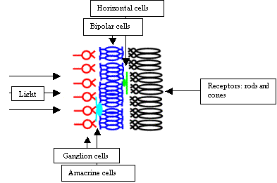Light entering the eye must pass through several layers of cells before it can reach the receptors. The image intercepted by the receptors is thus weaker and somewhat blurred. This would not happen if the order of the cell layers was reversed. The reason why it is the way it is, is unknown.

Information processing starts with the receptors. There are two types of them: the rods and the cones. The rods respond to dim light. The cones on the other hand need much brighter light. There are three types of the cones. These types differ in the frequency of light, to which they respond best.

Density of the rods and the cones is not uniform across the retina. The number of the receptors is about 120 million (corresponding to about 10000x10000 pixels, if the density of the rods and the cones were uniform). An elementary observation that in the dusk we see only black and white can be explained by the fact that in dusk only the rods are activated.

In the middle layer of the retina we can find bipolar cells. These cells receive input directly from the receptors and horizontal cells. Bipolar cells have interesting function. They can be divided into two groups; bipolar cells from the first group respond best to white circle with black surround. Bipolar cells from the second group respond best to black circle with white surround.

Figure: bipolar cells function:

Cell responds best to a white circle with a black surround. It doesn’t respond to a white circle with a white background or vice versa. We can say that this cell sums the inputs from the center circle and subtracts the inputs from the surround circle.

This behavior was first observed by Kuffler. He discovered this behavior on the ganglion cells (behavior is propagated to them from bipolar cells). This behavior was one of the reasons why scientists for a long time couldn’t measure anything reasonable on the ganglion cells (and thus on the eye nerve). They measured cell responses after flashing light to the cat’s eye. For the cells to respond, they need contours in the image, and contours are not created with illumination of the whole retina.

Information that passes through the eye nerve has to first pass through the layer of bipolar cells. That means that most of visual information passing to the visual center is reduced into contours. This can be demonstrated by a simple experiment with the blind spot. Blind spot is a location on the retina where the eye nerve forms. It lacks rods and cones, so we cannot see there. In the experiment, we can take for example blue paper with a small white spot on it. Then we need to look at it with one eye closed. Then move the paper slightly to the right (in the case of the right eye opened). In a moment the white spot disappears and on it’s place we will see blue paper (previously detected contours of the white spot are now missing).

Ganglion cells compose the last information-processing layer in the retina. They are much less numerous than bipolar or receptor cells (there are about 1 million ganglion cells).

Diagram for a ganglion cell:

Ganglion cell is red. It sums inputs from several bipolar cells. Ganglion cells are 100x times less numerous than bipolar cells.

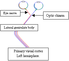
The axons (outputs) of these cells, grouped without apparent order, continue to the small unit named lateral geniculate body (LGB). While on the way, they cross; the axons of the ganglion cells from the left part of the retina from both eyes continue to the left hemisphere - to the left LGB. Symmetrically the ganglion cells axons from the right part of the retinas continue to the right hemisphere. The reason is not known. It’s interesting that visual systems in animals in many aspects differ. In animals with eyes not heading to the front as in humans but to the side as in birds, left hemisphere processes information from one eye and right hemisphere from the other eye. I will not describe function of LGB. Its purpose in visual information processing is not completely known and information passing through it is mostly unchanged.

3.3 The primary visual cortex

The primary visual cortex is approximately 2 millimeters wide and consists of 200 million neurons. It is probably the most explored part of the brain.

3.3.1 Simple cells

Simple cells receive input with characteristics of the output from ganglion cells. These cells respond best to lines with a specific direction. This behavior was discovered by Hubel and Wiesel in 1958 [1] (they received Nobel prize for this discovery). They found this behavior in other type of cells named complex cells. I will describe them below.

One of the possible figures for a simple cell:

A simple cell responds best to line with a specific orientation. It responds less or doesn’t respond at all to lines with different orientation or to other geometric objects.

The cells for all orientation are present (with distance about 10 degrees apart).

Possible wiring of a simple cell:

Inputs from the cells with characteristics of ganglion cells are summed. Cells should lie on a line.

3.3.2 Complex cells

These cells are most numerous in primary visual cortex. They also like simple cells respond best to the lines with specific orientation. The difference against simple cells is that complex cells indirectly process information from more receptors than simple cells. The other difference is that because of the adaptation on synapses, these cells are activated if the line with a specific orientation moves in a specific direction. That means that most of our visual stimulus consists of movements. This can be presented by one interesting observation. Our eye is regularly slightly moving (randomly and uncontrollably) to the sizes. When an image is artificially stabilized on the retina, so it is not moving, the image disappears and we cannot see anything [Riggs, Ratliff 1952]. After slight movement of the image, image appears again. This may imply that our ability to see static image was build by evolution on top of already functioning recognition of movements (to see and respond to movements was probably more important than to see static image).

3.3.3 End-stopped cells

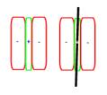
At last I would like to mention end-stopped cells. They similarly to complex cells respond best to a line with a specific orientation. The difference is that they respond only if a line has a specific length. These cells respond best to arcs.

Figure for an end-stopped cell

Cell responds best to the lines with specific length. It responds less or doesn’t respond if there is a vertical line in the red area (if the cell detects vertical line as the cell on the picture). These cells respond best to arcs, bends, corners etc. They respond only to the lines of one direction (line with this orientation must be present in the green area)

One of the possible wirings for an end-stopped cell:

The blue circle represents an end-stopped cell. The green color represents excitatory and red inhibitory connections. Wiring is theoretical. Real wiring is not known.

3.4 Summary

At the end I would like to stress: 1, I have mentioned only some of the cells in the primary visual cortex. Interesting are also binocular cells (cells receiving input from both eyes) and their function in stereopsis; or sharing of information between two hemispheres through corpus callosum, so we don’t see break on the middle of our visual field. More information can be found in [1]. 2, Although other types of cells with partial symbolic description are known, today it's assumed that it's not possible to continue with such a description to the end. We cannot expect to find a cell that recognizes our grandmother somewhere farther in the processing of visual information (so called grandmother cell theory). Information processing cannot be reduced to the function of one neuron. 3, Question about genetic predetermined wiring of primary visual cortex is not yet fully answered. Several experiments in the past have shown that if someone closes cat’s eye for some period after birth, cat would not be able to see with this eye for the whole life. It was shown that this is not result of that cat is learning to see after birth but it is more the cause of that binocular cells (cells receiving inputs from both eyes) adjust so they prefer input only from initially open eye. Theory that this wiring is predetermined genetically was strengthened by experiments with young macaques. Young macaque can see and has developed all types of cells described in this chapter on the first day after birth. Currently (to my knowledge) it is supposed that wiring is completed in mother’s uterus. Experiments don’t show if there is alternative to the known hierarchy of cells.

4. Creature’s structure

Layers

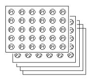
An evolved creature consists of layers. We can imagine a layer as a center for processing one characteristic of the image. For this purpose, layer can utilize inputs from other layers. Direct and also indirect recursion is allowed.

An equivalent to the layer in a computer language could be a function or a module.

Every layer consists of two-dimensional array of cells.

The cells of a given layer perform the same function. The cell in the layer A can utilize input from layer B. An important feature is that the cell on position [x,y] utilize inputs of cells with positions relative to the [x,y].

Layer with number 0 is predefined. It is not evolved. A cell on the position [x,y] in this layer contains 1 if there is a black pixel in the input at the position [x,y]; it contains 0 otherwise. The result of the recognition process for a given creature and given image is equal to the result of the middle cell in the layer 1.

New creature inherits layers of its parents. The task of the genetic algorithm is to ensure that good layers – the layers that are good in recognizing of some feature - will survive in the population. Layers can utilize abilities of other layers. That means that if one creature discovers better layer for say detecting of line segments and another creature improves its layer for detecting curvatures, these two layers will, thanks to genetic algorithm, meet in a new creature. We can imagine this as developing object-oriented application. These objects are improved. Due to the genetic algorithm there is a tendency that the good versions of these objects will meet in a new creature / application.

4.1 The code for the layer

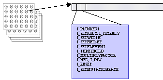
The code for the layer consists of a sequence of simple instructions. It consists of a sequence of integer numbers. The interpretation of the code is similar to the interpretation in modern computers. The first number is a type of the instruction. If this type of instruction has parameters, the following numbers in the code are taken and the instruction is performed. Instruction counter is incremented and subsequently next instruction is performed. The results from instructions are accumulated. The result of code interpretation is single integer number.

The representation of a type of an instruction doesn’t differ from the representation of instruction’s parameters. Both are simple integer numbers. The consequence is that if the code for the layer is shifted, it is very likely that the meaning of the code will totally change. It’s possible that parameters of an instruction will become instruction types and conversely an instruction type can become a parameter.

The basic characteristic of the language is that instructions have few parameters. The reason for this is that otherwise it would be very difficult for the genetic algorithm to develop meaningful code. It would be difficult to set up an instruction with many parameters. In the current implementation of the language it’s possible to set up parameters prior to the given instruction. That means that if instruction A needs two parameters P1, P2, there are two instructions „Set P1“, „Set P2“ that can be used anywhere prior to using the instruction A. If they are not used, P1 and P2 have default values. Advantage of this implementation is that instructions “Set P1” and “Set P2” don’t need to have exact positions in the code (“Set P1” can be located before “Set P2”, or vice versa). This results in more freedom for the genetic algorithm.

For example the instruction I_PLUSRECT for summing rectangle of inputs from different layer needs these parameters:

A, layer from which to sum

B, relative position (to current cell) of the rectangle

C, dimensions of the rectangle

For this purpose there are special instructions in the language: I_SETWIDTH, I_SETHEIGHT, I_SETRELX, I_SETRELY, I_SETELEMENT. These instructions can be used anywhere in the code before the instruction I_PLUSRECT.

In the proposed language I tried to introduce as few instruction types as possible. The objective was to have few instruction types that can describe simplified function of cells in early visual pathway. As the limitations of the instruction set is more understood, new instruction types will be added.

Types of instructions and description of their purpose:

I_PLUSRECT: Instruction sums rectangle of inputs from the specified layer. It adds this number to the current code’s intermediate result. The rectangle’s position is set relatively to the current cell.

I_SETRELX, I_SETRELY: Set relative position of the rectangle summed by I_PLUSRECT.

I_SETWIDTH, I_SETHEIGHT: Set dimensions of the rectangle for I_PLUSRECT. As in the case of I_SETRELX and I_SETRELY also these instructions can be used anywhere and in arbitrary order in the code before I_PLUSRECT.

I_MULTIPLYFACTOR: This instruction modifies the weight of the inputs for I_PLUSRECT. Every time I_PLUSRECT instruction is performed, the result sum of the inputs is multiplied by a so called multiply factor. This instruction modifies multiply factor by multiplying it with rational numbers 1/3, 1/2, 2 or 3.

I_SETELEMENT: Sets the layer from which I_PLUSRECT sums. This instruction can lead to direct or indirect recursion. Computations that would lead to cycle are eliminated (their result is 0), on the other hand computations that compute shifting rectangle that in short time crosses border of the cell layer are handled correctly.

I_SETMUTATIONRATE: Changes mutation rate of the part of the code behind this instruction. See section about genetic algorithm parameters.

I_THRESHOLD: If the number summed up to now is greater then or equal to the parameter, this instruction replaces summed number with 1. Otherwise it replaces it with 0.

I_NEG: If the number summed up to now is equal to 0, after this instruction it will be 1. It will be 0 otherwise.

I_INV: If the number summed up to now is equal to n, after this instruction it will be –n.

I_RESET: Resets information set by I_SETRELX, I_SETRELY, I_SETWIDTH, I_SETHEIGHT and all previous I_MULTIPLYFACTOR instructions.

5. New creature

New creature is created by combining layers of its parents. The probability that a specific layer will be inherited is equal for both parents and so it doesn’t depend on their success in recognizing patterns. Crossing on the level of single layer also happens with some probability (crossover). In this scenario a random position in the layer is chosen. The code of the layer is divided on this position. The beginning is taken from one of the parents. Tail is taken from the other parent. Observations confirm that this feature significantly increases efficiency of the genetic algorithm. New layer is with some probability modified (mutated). These modifications are of several types.

5.1 Mutation types

Simple mutation: The code is modified with a small probability on random location.

Shift: Code of the layer is on some random location shifted to the left or right. This results in shortening or extending of the layer’s code. The shortening/extending is one gene word long. The meaning of the part of the code after this location can change. Length of the code is restricted and the code cannot be extended above this number.

Split: The result of a split is a new layer. Some existing layer is taken and it is divided on the random location. New instructions are added to the first part of the divided layer. These instructions reset rectangle position to 0,0 and dimension to 1,1 and sums rectangle from the new layer. That means that the input on the current position from the new layer will be computed. The second part of the code from divided layer will become the code of a new layer. Thus the new cell will compute something similar or equal (not always, because relative position set by I_SETRELX etc. are not transferred between layers) to the previous version of the cell on that position. The number of the layers is bounded.

Delete: Deletion of a layer. The first two layers cannot be deleted.

5.2 Genetic algorithm’s parameters

In designing of the genetic algorithm we cannot bypass the problem how to set up it’s initial parameters. That includes parameters like the frequency of mutation, the shift of the gene etc. One of the possible solutions is to try various combinations of these parameters and following the comparison and selection of that, which seem to be the most successive. This technique has been used. Disadvantage of this technique is that for different problems – that means the problems of recognizing different objects – the ideal parameters of the genetic algorithm can be different. The problem of fixing ideal parameters is even deeper. The optimal rate of mutation can differ also in various phases of development of creatures. At the beginning the optimal rate of the mutation is higher, however later lower rate of the mutation can be optimal. The same applies to the different layers. Theoretically optimal rate of the mutation can differ also in different parts of the code of one layer.

I decided to address this problem also with different technique. The designed language contains instruction, which allows modifications of the mutations frequency. That means that genetic algorithm evolves creatures and inside of them it evolves also it’s own parameters. Specific instruction for changing mutation rate is located somewhere in the code. This allows genetic algorithm to change its parameters only in some specific part of the code. Concrete example can be: if one layer is good in recognizing of some pattern; the mutation rate of this layer should be ideally lower than the mutation rate of the part of the different layer, which is not yet so successful. That means that the mutation rate of older, more tested layers should be lower than mutation rate of newer layers.

This kind of genetic algorithm’s parameters evolution can also serve as indicator, that we should change initial parameters of the genetic algorithm. For example if there is the instruction for change of mutation rate at the beginning of the most codes of the layers after some time, we know that initial parameters should be different.

It's possible that similar technique was used by nature while evolving animals, including humans. The principle is based on so called stuttering genes. These parts of the chromosomes increases chance that reproduction of chromosome will error, and genes behind the stuttering sequence will be shifted, which will in turn change following genes meaning. Interesting article on this issue with examples is [4].

6. The inputs

The creature’s success and so its probability to have offspring depends on it’s ability to recognize patterns. Patterns are represented by small black and white images. All creatures in a population receive the same input. If a creature correctly classifies given pattern, it receives one point. Patterns are taken from pre-generated set of patterns. In some tests I generated inputs in runtime. After finishing all rounds of testing; the success of the creature is equal to the number of points it earned. The best creatures are remembered throughout the history for later examination.

7. Testing and the observations

Today we can be sure about the usefulness of structuring creatures into the layers. It became apparent that the genetic algorithm often uses this feature. For example also on such a simple pattern as a cross, the genetic algorithm chooses the way with two or more layers recognizing horizontal and vertical lines. The cross is recognized by combining inputs from these two layers. This applies also to arc (in this case recognizing is similar to the function of end-stopped cells). The reason behind this behavior is that the code for the layer, to able to be generated by the genetic algorithm, must be short. The consequence is richer hierarchy of the layers.

One of the observed problems is tradeoff between fast generation of a small population and tendency of such a small population to loose acquired abilities. From the observations, I’ve concluded that it is useful to evolve more than one population simultaneously. One of the populations should be smaller. These two populations should regularly exchange their best members. The bigger population can be evolved slowly and can serve as a “backup” of acquired abilities.

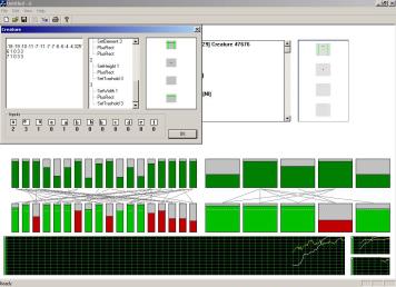The problem I am facing today concerns creation of new layers. Everything works above expectations if creatures are trained with the help of human. For example let’s assume that pattern A can be recognized by recognizing two simpler patterns B and C. The easy way (which is working) is to train creatures to recognize patterns B and C and then (when they are good on B and C) switch to pattern A. The other way, that is problematic today, is to give A on the input and wait that the layers for B and C will evolve. Today genetic algorithm is successful in this scenario only on very simple patterns.

8. Summary

This paper gave overview about one possible approach to the pattern recognition problem. Although it doesn’t aspire to be directly useful for practical problems in image recognition in near future, I think that ideas and observed features can be inspiring and help while dealing with real problems.

9. References

[1] Hubel, D.: Eye, Brain and Vision, Scientific American Library, 1995

[2] Marr, D.: Vision, W. H. Freeman and Company, 1982

[3] Goldberg, D.: Genetic Algorithms in Search, Optimization and Machine Learning, Addison-Wesley Pub Co, 1989

[4] Moxon, R., Wills, Ch.: Scientific American, January 1999

[5] Fukushima, K., Wake, N.: Handwritten Alphanumeric Character Recognition by the Neocognitron. IEEE Transactions on Neural Networks, 355-365, May 1991