Towards Optimal Combination of Shooting and Gathering Stochastic Radiosity

Martin Balog

7balog@st.fmph.uniba.sk

Faculty of Mathematics, Physics and Informatics
Comenius University
Bratislava / Slovakia

Abstract

This paper deals with combination of shooting and gathering stochastic radiosity methods. The basic two-pass methods are reviewed and other new methods are proposed. The fundamental motivation for this paper is to develop an iterative two-pass stochastic radiosity that provides the progressive refinement feature of both types of radiosity algorithms. We want to give the user a new, better, solution of the radiosity problem that improves incrementally over the previous one.

Keywords: shooting radiosity, gathering radiosity, two-pass methods, progressive refinement, Monte Carlo.

1. Introduction

Digital image synthesis is very wide area in computer graphics. Trying to provide images of virtual environments we have many choices how to achieve the goal. One way is a photo realistic image synthesis. In this type of image synthesis we want to create the picture that looks like a photograph of a real scene as much as possible. One of the main problems in this field is to simulate the realistic lighting. Without the light there is no image and with non-realistic lighting models we can even confuse the user. Therefore for realistic image synthesis we have to simulate the light very accurately.

The radiosity method belongs to a family of global illumination algorithms. It is a simplified version of the rendering equation proposed by Kajiya in [Kaji86]. It makes this equation been trackable by reducing it to a simpler form using some assumptions about the input scene. Very good book on radiosity is [Cohe93] where you can find all the necessary background information on radiosity.

We can divide the radiosity methods into two groups. Deterministic methods are solving systems of linear equations to compute the illumination in the scene while stochastic radiosity methods are based on the Monte Carlo integration. This paper deals with possible combinations of different stochastic algorithms to obtain better results for the radiosity. The paper is organized in the following form. First we review several stochastic radiosity algorithms. The second section deals with progressive refinement methods and two-pass methods that are very useful and effective. The third section proposes new possibilities of combination of different stochastic radiosity methods. Several experiments and their results are presented. Finally we make some conclusions about what does our approach bring to users.

1.1 Shooting versus gathering approach

Shooting and gathering radiosity are two opposite ways of solving the system of linear equations. Gathering radiosity can be found in classic Gauss-Seidel iteration methods for solving systems of linear equations. It means that the illumination of a patch is gathered onto the patch from the surrounding environment. The system is solved (has converged to a solution) when the difference between two iterations (gathers) is lower then some predefined threshold.

On the other hand shooting approach, usually called progressive refinement radiosity, tries to simulate the light transport from the light sources. It introduces new value for each patch, the unshot radiosity. It starts with source patches having their unshot radiosity equal to their emission. A patch is chosen and its unshot radiosity is distributed into scene. This reduces the unshot radiosity of source patch to zero but increases the unshot radiosity of hit patches. When the reflection is lower then 1.0 for each patch, the overall unshot radiosity is reduced with more shootings. Shooting has one nice feature. After only few steps the primary illumination can be computed thus giving us good approximation of the final solution. Shooting radiosity is finished, when the total unshot radiosity over all patches is lower then some predefined value. This kind of solution is actually Southwell iteration for solving systems of linear equations. Although it is not efficient for systems common in other applications, in radiosity it is a good choice.

1.2 Stochastic radiosity (Monte Carlo radiosity)

Stochastic radiosity is based on Monte Carlo integration. The light transport in stochastic radiosity is done by the means of rays. Rays are abstraction of photons. The basic advantage of Monte Carlo radiosity methods over deterministic ones is the there are no form-factors computed explicitly. This saves a lot of computations, because the form-factors need information about mutual visibility of patches that is extremely hard to compute. The role of form-factors is replaced by the probability that a ray shot from a patch reaches the other patch. Thus the form-factors are only computed implicitly. In addition, in deterministic methods form-factors are computed between all patches, while in MC only between mutually visible patches. This is highly important especially in complex scenes. However this is at the expense of having solution with variance from a correct one. Every time we run the computation we get a different solution. There are either shooting or gathering Monte Carlo radiosity algorithms. In both cases rays are cast from patches to send/receive light energy. Because we assumed that surfaces are made of diffuse materials, their directional distribution is always cosine according to the angle between ray and normal of the surface at the ray origin.

1.3 Shooting stochastic radiosity

Shooting stochastic radiosity is based on shooting the unshot radiosity of patches into the scene and transferring the power to other patches. In the whole paper we will refer to an unshot radiosity as a part of the radiosity of the patch that wasn’t accounted into the solution yet. All the energy transport is based on power that is computed as radiosity of patch multiplied by its area. For a patch P_i with unshot radiosity dB_i a number of rays is chosen and energy of each ray is computed as dB_i*A_i/n_i. Then n_i random directions are chosen according to cosine distribution. For each direction we send one ray and find the nearest hit surface. We multiply the energy of that ray by reflectivity of hit patch and add its influence to the radiosity and unshot radiosity values of the patch. Then we set the unshot radiosity of the shooting patch to zero. We repeat this process until convergence, which is defined by a threshold value of overall unshot radiosity.

Good idea about the shooting stochastic radiosity is to make each ray do the same amount of work thus decreasing the computation in situation were the contribution of source patch is too small. This was very well discussed in [Feda93]. Some additional advantages of this approach are also discussed in the progressive ray refinement radiosity chapter later on.

1.4 Gathering stochastic radiosity

Gathering stochastic radiosity uses different approach. Instead of a patch shooting its energy into the scene, it gathers its illumination from the scene. The whole process works in steps where in one step each patch gathers its new illumination value from the present values (temporary solution) and uses these values as input for next step. The convergence is defined as threshold value of difference between two consecutive steps. Again, for each patch we choose number of rays and we send them according to the cosine distribution into the space. The average value of radiosities of hit patches multiplied by the patch reflectance is the value of radiosity of the gathering patch for the next round. Typically for each patch we choose the same number of rays during the whole computation.

1.5 Two pass methods

Two-pass radiosity methods are designed to run in two consecutive steps. Typically the first step is a shooting radiosity followed by second step, gathering radiosity. Let’s have a look at reasons why such algorithm is useful.

Shooting radiosity by sending rays from patches can miss many small destination patches. This kind of error is increasing with the scene complexity, when many patches are created. Therefore we need to use many more rays to get a good solution. However when a larger patch is between small, this one is highly over sampled and we waste computation time and can also create visible artifacts (bright spots). Gathering radiosity never misses any destination because it computes radiosity for each patch. On the other hand sampled directions used for gathering can miss an important light source. Especially when a small patch has high radiosity and thus has high importance on the illumination of the scene, the gathering can loose.

Problem found in one of the radiosity algorithm is solved by the other. Therefore two-pass methods are being used. First the shooting is used to distribute the light from light sources into the scene. Although its results aren’t very good for human perception, it provides a good overall light distribution. With some precision it simulates the light interreflection in the scene. But the variance of the solution is high thus difference in the illumination between neighboring patches is also very high in early shooting solutions. To make it smoother we can use the gathering radiosity. We use the result of shooting as an input for the gathering step. This helps to solve the problem of missing patches. Radiosity of all patches is computed with the same number of rays for each patch so the overall accuracy of the solution depends only on the accuracy of the shooting solution and the number of rays used for gathering. When we gather from a complete shooting solution we still have the problem, especially in direct illumination, that we can miss some important patches. The quality of direct illumination is a well-known problem in all Monte Carlo algorithms. There is a possibility to divide the gathering into two parts, one for direct and one for indirect illumination only. For more details please refer to [Shir91].

The second step, the gathering, can be done in more ways then just on a per patch basis. For smooth illumination reconstruction at least a linear interpolation of vertex radiosity values is used. Vertex radiosity is normally extrapolated from patches as area weighted average. The gathering radiosity step gives us the possibility of gathering radiosity directly in the vertices and thus avoiding the need of extrapolating the radiosity values. This gathering solution stays in the object space, as the per-patch gathering does. Other possibility is to gather radiosity per pixel. A small virtual patch is found (typically only points are used) that can be seen through a pixel and radiosity is gathered for this virtual patch. This approach can solve many problems of all radiosity algorithms. We don’t need to deal with the discontinuity meshing; no smoothing of radiosity is needed. However it moves the solution from the objects space into image space. Because of this we will not use this type of gathering in this work. We will work with the per-patch gather exclusively.

2. Progressive refinement approaches

Because the radiosity values of patches computed by Monte Carlo methods behave like a random variable with only an expected value we never get the same solution twice on the same input scene. The difference of the solution from the correct one can be expressed via variance. The goal is to reduce the variance as much as possible. Having two complete solutions of radiosity we can combine them into one even better with lower variance. All we need is a good weighting [Sber95]. As Shirley in [Shir91a] presented, the variance of a single solution is dependent on the number of rays used (in the shooting the number depends on the energy each ray is carrying). The weighting in single pass radiosity can be determined from these values.

2.1 Progressive ray refinement (PRR) radiosity

In [Feda93] Feda et. al. presented a radiosity algorithm that incorporates the feature of refining complete radiosity solution. It shows how to refine a previous solution by adding more rays. The number of rays depends on the amount of energy each ray is carrying in each phase of calculation. The weighting is inversely proportional to the energy of single ray. This results in a following algorithm:

Do a coarse shooting with relatively big energy carried by a single ray

Until the quality is not satisfactory

Reduce the energy carried by a single ray

Compute a new solution of shooting radiosity

Combine this solution with the one already provided according to the energies of rays and update the values

Algorithm 1. Progressive ray refinement stochastic radiosity

PRR radiosity is one of the first algorithms that can provide improvements to the radiosity solutions as the time progresses. This gives a good quality control to the user. This feature is the most important we will try to incorporate into the new algorithms presented in this paper

2.2 Progressive refinement gathering radiosity

This gathering radiosity algorithm is actually a two-pass method. Instead of using its previous solution as input to the next iteration step it uses a complete shooting radiosity as the input.

The gathering starts with a coarse gather step with low number of rays per patch. It computes just one step of gathering from the provided solution and returns this as a complete solution. Notice that there are all the interreflections already counted in it, because the shooting computed them already. Thus we only need one gathering to have full solution of specified accuracy (depending on the number of rays used). When the user decides that it is not good enough s/he can start next gather with new number of rays and combine it with the previous one. Technically it is like adding more rays to the simulation thus increasing accuracy. The pseudocode is written in the Algorithm 2.

Get a shooting radiosity solution.

Do one gathering round with some number of rays per patch.

Until the quality is good do the following

Choose the new number of rays for next gather round.

Gather radiosity from the initial shooting solution.

Combine the new gathering solution with the previous one

Algorithm 2. Progressive gathering stochastic radiosity

Combination of two gathering rounds starting from the same shooting solution is straightforward. The weighting is proportional to the number of rays used for gathering radiosity of single patch in each step. With such gathering algorithm we have to take into account that using only few rays for gathering we can get much worse solution than the initial shooting gives us. One has to be very careful by setting the number of per-patch rays for gathering. Therefore progressive refinement is great option for quality control.

The gathering radiosity has the same good refinement feature as the previous shooting radiosity algorithm. But there is a problem. First you have to compute at least some shooting radiosity to provide the light distribution in the scene. The gathering iteration steps are computed in equal time period, but the shooting step introduces some initial computation that lacks this feature. In the next chapter we will try to solve this problem.

3. Iterated two-pass stochastic radiosity

In this chapter we will introduce two new approaches to two-pass radiosity. The goal is to design a two-pass algorithm that can progressively refine its previous solutions. The reason is that the two-pass radiosity solves some problems found in single pass radiosity algorithms. On the other hand it lacks the possibility of getting a coarse solution for preview and then refining it for higher quality without loosing the computation time spent on the first solution. This is the basic expectation we have on the algorithm.

The first approximation has already been proposed. It is the progressive gathering radiosity. This is not exactly what we need, as it prohibits from enhancing the input shooting radiosity solution.

3.1 Progressive two-pass radiosity

This algorithm is very similar to the progressive refinement gathering radiosity. The only and basic difference is that in the previous version, the shooting radiosity solution was computed at the beginning and than during the gathering refinement there was no change in the quality of the shooting solution. The shooting was computed with some predefined quality (based on the per-ray energy settings). If we wanted a higher quality for the shooting input we needed to setup such quality already at the beginning and wait for its computation. However even if we use PRR radiosity for shooting it is not a progressive two-pass radiosity.

We can solve this problem using an approach described by the schematics on the Figure 1. If we can do gathering from early stages of the refining shooting solution, we can solve the probem of initial computation. We need a new weighting for two gathering solutions from different shooting inputs. For the purpose of designing it we have ran several test computations on different scenes.

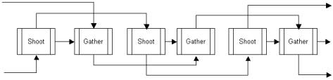
Figure 1: Block diagram of the Progressive Two-pass Radisoity algorithm .

We ran a precise gathering step from different shooting solutions. The results of the shootings were improving for each computation while the number of gathering rays was the same. The Figure 2 shows the RMS error of the gathering solution based on refining shooting radiosity solutions. We used two approaches. One series of test was computed with and one without the ambient term added to redistribute all the unshot radiosity that the shooting wasn’t able to process anymore.

Figure 2: The RMS error of the gathering radiosity computed from refining shooting solution. You can see that using the ambient term allows us to use the weighting proportional to the number of rays also in our algorithm without any consideration about the input shooting radiosity quality.

As you can see in the non-ambient version, from some point the gathering quality was nearly the same without any improvements as the iteration process progresses. The initial increase in the RMS was due to a low quality of the shooting radiosity. The per-ray energy was too large to be able to distribute the light through the scene. Much of it was left in the unshot radiosity values, because the values on patches were too low to emmit at least a single ray. From the point where the number of rays used for shooting was large enough to give solutions with the same percentage of unshot radiosity from the total radiosity in the scene, the quality of gathering step was not increasing with the quality of shooting. The threshold value of unshot radiosity was set to 1%. In the radiosity with ambient term used for final energy redistribution the initial RMS increase was very low, actually only in absolutely poor solutions. Nearly all tests have shown the same RMS error from a reference solution. Figure 3 is showing some results for a Cornell box scene.

Figures 2 and 3 show that if we gather from two different shootings we don’t need to count the different quality of the inputs and the weighting is the same as in progressive refinement gathering radiosity (chapter 2.2). The only requirement is that both shootings have to distribute nearly all of the energy in the scene or we have to use the ambient term to redistribute the remaining energy. We cannot forget that if we don’t distribute nearly all the energy, the gathering step will provide a smooth, but darker solution. It will lack the unshot radiosity that it can’t count in.

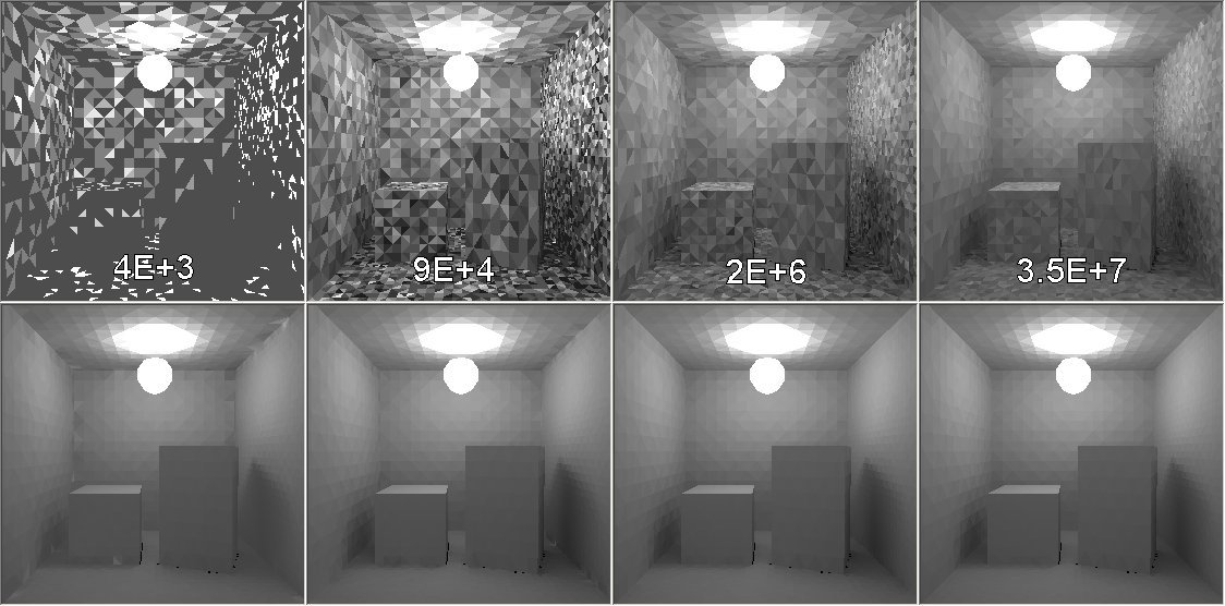
Figure 3: The results of test on a Conell Box scene. The upper row of images shows improving shooting solutions with ambient term and the number of rays used while the lower one is made of gathering solutions from above shootings. You can see that even the quality of shooting is low, the gathering gives nearly the same results. There were nearly 8E+8 rays used for each gathering.

This observation of gathering solution quality let us write the following algorithm:

Compute initial shooting solution

Use it as input for gathering step with some per-patch ray count.

Until the quality is satisfactory do the following

Compute new shooting step

Combine it with the previous one

Use this refined solution as input for next gathering with new number of gathering rays.

Combine this gathering step with the previous one depending on the per-patch ray counts

Algorithm 3. Progressive two-pass radiosity

3.2 Iterative Combined Monte Carlo Radiosity

The previous algorithm posses the progressivity, efficient energy distribution by shooting and smooth illumination by gathering featured by the two-pass radiosity methods. As already discused in the chapter 1.5 both radiosity algorithms have problems dealing with the direct illumination. We have mentioned that it is very useful to divide the computation into two steps, for direct and indirect illumination [Shir91]. Note that looking at the gathered picture we can see that in the indirect illumination the gathering radiosity is much better. Even when using coarse shooting step for input to the gathering, the indirectly illuminated parts of the scene are very good and smooth. On the other hand, the direct illumination in the shooting approach behaves little bit better than in gathering (Figure 4). It shows that with using a direct combination of shooting solution and gathering solution into one, we can dramatically enhance the quality of at least the indirectly illuminated parts of the scene. Further more, for highly complex scenes the gathering step can produce much smoother solution even with fewer rays than the shooting does.

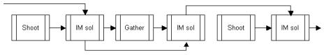
Figure 5. Block diagram of the Iterative Combined Monte Carlo Radiosity

This algorithm uses an intermediate solution that is converging to the result. We switch between shooting and gathering steps and their solutions are added (combined) to the intermediate solution to improve it. The improving solution is also used as the input to the gathering steps. Combination of empty intermediate solution and any other (shooting) is simply an assignment.

The last computed combined solution is always used as an input to the gathering. The convergence criterion can be defined as reaching a threshold value of difference in radiosity of patches in consequent iterations. A prove that the combined method converges to the correct solution is not available yet. But if the error can be controled, the algorithm should theoretically bring better convergence rates than any usual single/two-pass stochastic algorithms before. The basic problem with it is the combination of shooting and gathering solutions into one. This has to be done very carefully. It is clear that both radiosity solutions of the same scene have the same expected value. Therefore the combination is possible. The problem is that we want to reduce the variance as much as possible to speed-up the convergence. As in the PRR we need to develop a good weighting of solutions based on the parameters of simulation of either shooting or gathering or combined radiosities.

We initiate an empty intermediate solution (IM)

Repeat until convergence

Do a shooting solution with defined per-ray energy

Combine this shooting with IM solution

Do a gathering from actual IM solution

Combine this gathering with the IM solution

Update the parameters for shooting and gathering

Algorithm 4. Iterative Combined Monte Carlo Radiosity

At the moment we will not present any real solution to the weighting for this combined radiosity method. We just want to present some basic ideas about what we have to keep in mind and what could be the way to follow when looking for the solution. This is a problem for a future work.

As we already saw even a good shooting solutions is useless when we use few rays for gathering. Bad combination of such solutions could destroy the final results. A good idea for solving the weighting problem could be a definition of radiosity solution accuracy that can express the correctness of either shooting or gathering radiosity in a compatible way. Having such accuracy measurement the combination weighting could be derived from it. In general the quality of Monte Carlo radiosity depends on the number of rays used for the simulation. One possible way of accuracy measurement is to count the total number of rays used during the computation. But because of the absolutely different usage of rays in each algorithm we have to check whether one ray for shooting has the same importance on the quality as for gathering. It means that if we use some number of rays for shooting and then the same number of rays for gathering, we have to compare the quality we have got.

4. Conclusions

Two-pass radiosity is showing to be very efficient in terms of convergence and perceptual quality, because it generates very smooth and visually plausible results. It also helps to solve some problems of high density meshing in complex scenes. In this paper we have presented two new designs of two-pass radiosity algorithms. The first method introduced the progressive refinement into two-pass stochastic radiosity. The results show that we don’t have to design new special weighting for refinement of two-pass methods. The output images are perceptually very good much sooner during the computation. Progressive refinement is very important for users who want to be able to control the quality precisely, because the radiosity computations are still very time consuming. We believe that the Iterative Combined MC radiosity should be a hopeful algorithm, but we still din’t implement it thus there are no real results about it. We have to do more research in this field to check all its possibilities and advantages.

5. Acknowledgement

I want to thank everyone who helped me writing this paper, especially Mr. Pavol Eliáš, my diploma thesis supervisor, who helped me getting into the field of stochastic radiosity and gave me many valuable advices and reviewed this paper. I also want to thank Mr. Andrej Ferko for his support and help he gives to the students of computer graphics at Comenius University in Bratislava. Finally I want to thank my parents for their love and support they gave me.

6. References

[Cohe93] Cohen, m., Wallace, J.: Radiosity and realistic image synthesis, Academic press Professional, 1993.

[Elias] Eliáš, P., Purgathofer, W.: Monte Carlo radiosity: Comparison study.

[Elia00] Eliáš, P.: Stochastic radiosity methods, Master’s thesis, Comenius University in Bratislava, 2000.

[Feda93] Feda, M., Purgathofer, W.: A progressive ray refinement for Monte Carlo radiosity, in Proc. of the 4th Eurographics workshop on rendering Paris, France, 1993.

[Glas95] Glassner, A.: Principles of digital image synthesis, Morgan Kaufman publisher, 1995.

[Kaji86] Kajiya, J.: The rendering equation, in Computer graphics, Proc. of Siggrph’86, vol.20, No.4, 1986.

[Patt92] Pattanaik, S., Mudur, S.: Computation of Global Illumination by Monte Carlo simulation of the Particle model of light, 3rd Eurographics workshop on rendering, Bristol, England, 1992.

[Sber95] Sbert, M., Perez, F., Pueyo, X.: Global Monte Carlo: A progressive solution, Rendering Techniques’95 (Proc. of the 6^th Eurographics Workshop on Rendering, Dublin, Ireland), Springer, 1995.

[Shir91] Shirley, P., Wang, Ch.: Direct lighting calculation by Monte Carlo integration, In Proceeding of 2^nd Eurographics workshop on rendering, 1991.

[Shir91a] Shirley, P.: Time complexity of Monte Carlo Radiosity, in Proc. of Eurographics ‘91, North Holland, 1991.

[Shir94] Shirley, P., Sung, K., Brown, W.: A ray-tracing framework for global illumination, in Graphic Interface ‘91, pages 117-128, June 1991.

[Shir94] Shirley, P., Chiu, K.: Notes on adaptive quadrature on the hemisphere, Technical report no. 411, Department of computer science, Indiana University, 1994.

[Shir] Shirley, P.: Hybrid radiosity/Monte Carlo Methods.

[Szir00] Szirmay-Kalos, L.: Monte-Carlo methods in Global Illumination, Script, Institute of Computer Graphics, Vienna University of Technology, 2000