Abstract

This paper proposes several algorithms to compute the 3D sound-field in complex environments. The basic idea is to explore the similarities of light and sound propagation and take advantage of efficient rendering algorithms and hardware to compute the sound field. First we consider only the direct effect of sound sources. Then single reflections of the sound are also computed using the analogy of local illumination models. The main problem in establishing such an analogy is that the effects of different sources emitting different sound waves cannot be added. Instead we have to keep the information from which source this sound was emitted.

Keywords: 3D Sound-field, Multichannel Sound, Image-based Sound Generation, Image Synthesis, Image Processing, Waveform

1. Introduction

At the dawn of the history of movies, the sound was mono then became stereo. Nowadays the sound is surround, which is either recorded or computed and finally restored by directed speakers. Meanwhile, images rendered by computer graphics algorithms have become more attractive and more efficient algorithms and image synthesis hardware have come to existence [1]. The main objective of this paper is to propose methods for realistic sound computation using computer graphics and image processing techniques. This approach has two merits. On the one hand, efficient image synthesis algorithms and hardware can be utilised for sound synthesis. On the other hand, the correct correspondence of the animation and the sound can be obtained automatically. The sound has similar properties as the light. The sound is also a wave that originates at sources, travels in space and scatters on surfaces as light does. If the sound waves are simulated by light, we can visualise the sound field. So every sound-source and sound-reflecting surface is interpreted as a light-source and light-reflecting surface, respectively. The intensity of the sound wave is proportional to the intensity of the light ray. Generating images from the location of the observer, we can describe the sound field of his environment. Taking into account the sound direction and spread, and computing only single reflections, these images allow sufficiently realistic sound generation.
In order to compute the sound field, the light equivalent of the sound is determined for every pixel or pixel-group in the image. The volume of the sound wave is proportional to the intensity of the pixels. The sound-samples which are coming from different pixel-directions are weighted according to the direction of the speakers. We have examined two methods for the waveform generation. The first method uses rendered images and obtains the required information only from these images. The advantage of this approach is that we can use off-the-shelf image synthesis algorithms and should use only simple image processing to find the sound field. Consequently, this method is fast and easy to implement. The second proposed method, on the other hand, uses the 3D definition of the scene and implements the complete light and sound rendering pipeline simultaneously. The second method is also able to produce Doppler effect and is more realistic. However, the price of the higher realism is the increased computational cost.

2. Importance functions of the sound channels

The sound wave is equivalent to the time function of voltage amplitude. The waveform is stored in a WAV file in digitized PCM (Pulse Code Modulation) format [16]. The loudness is depending on the power of signal (P), consequently it is directly proportional to the square of voltage amplitude (U²):

where U is the voltage amplitude and Z is the impedance of the system. Directing a sound wave in a stereo system into a specific direction, the signal amplitude is weighted according to the direction of the speakers. The multipliers of direction weighting are called importance-functions. The latent range of importance-functions is between zero and one. If there are more than two channels, i.e. we have at least a quadraphonic system (see Figure 1), then we can represent the whole sound field that surrounds the listener. In this case, we have to define the importance functions of the other channels. The importance functions must be interactively controllable because the position of the speakers can be altered at any time.

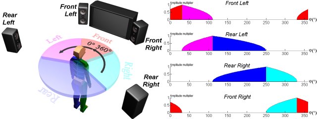
Figure 1: Quadraphonic sound system and its importance functions

3. Simulating the sound with light

In this section we examine, which visual rules shall apply to get the information of the sound from the rendered images. The primary questions are which and how many colours are used, and how we can mix them in the bitmaps to identify the sound sources unambiguously. We consider two rendering models. In the first model, no light (i.e. sound) reflection is allowed and the anti-aliasing is turned off. This means that we do not take sound reflection into account. In the second model this limitation is lifted.

3.1 Rendering with no reflection and without anti-aliasing

Suppose that we use different colours to identify the sound sources, mute objects and sound absorbers. If no light reflection is allowed and the anti-aliasing is turned off, then the image can contain only the own colour of the objects, thus they can be trivially recognised in different pixels (see Figure 2).
The problem of these settings is that only the sound source objects can be recognised and thus heard. Since other objects do not reflect the sound, the result is not realistic. Moreover, the minimal size of the small or far distant objects are limited by the pixel size. Objects having smaller projected size may appear and disappear in an unpredictable way.

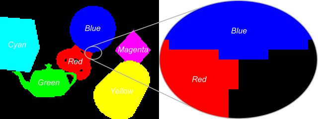
Figure 2: Using colours to identify sources. If no reflection and anti-aliasing are allowed, the colours distinguish the sources from each other.

3.2 Rendering with reflections and anti-aliasing

In order to compute more realistic sound fields, the reflections on the object surface should not be ignored. To allow light reflections, the material of these surfaces is set to reflect some portion of the incoming energy. Light reflection causes the colours to mix additively. Anti-aliasing, which is needed because of the poor resolution, also results in mixed colours (see Figure 3).
However, when the colours are mixed, we are not able to identify the respective sound sources from the pixel values. Suppose that we identified the first source with green, the second with red and the third with yellow colour. Assume that in one pixel we find yellow colour. Obviously, this might mean either that in this pixel we hear both the first and second sources or that only the third source can be heard here.

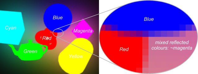
Figure 3: Using colours of the objects when reflection and anti-aliasing are enabled.

There are two ways to separate the sources. The first considers only one sound source at the same time and renders as many images as sources exist. In this case we work in grey-scale mode.
The other possibility is to turn to RGB mode and follow three sound sources in parallel. This time we identify the sound sources with the three base colours (Red, Green, Blue) (see Figure 4). These colours can only be used in true colour mode. We prefer the second method, because this requires less computation.

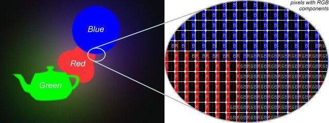
Figure 4: Using three colours (R, G, B), reflection and anti-aliasing. The effects of only three sound sources can be separated.

4. Image based sound field computation

Taking a photo of our entire environment, we have to use as many perspective images as main directions exist. These main directions are usually classified as front, back, left, right, top and bottom. These perspective images should be mapped over a sphere surface, viewed from the center of the sphere. On the other hand, we use six cameras looking at the main directions, their aspect ratio is 1:1 and their "angle/field of view" (FOV) is 90 degrees. The six views (the six rendered images) are on the six sides of a cube that is in the same position as the sphere. The surround speakers are usually in one plane (in the level of the listener's head), so we can distinguish only the "left-right" and the "front-back" sound directions. Using this sound system, we can feel the "top-bottom" direction only by special distortion of the sound. Therefore we use only the four horizontal images of the "view cube" and the top and bottom images are ignored (Figure 5). Of course, this is a big loss, because we have thrown away the third axis of the sound field description. However, we can correct this error by increasing the horizontal view of the cameras. But in this case the aspect ratio of the images will be changed.

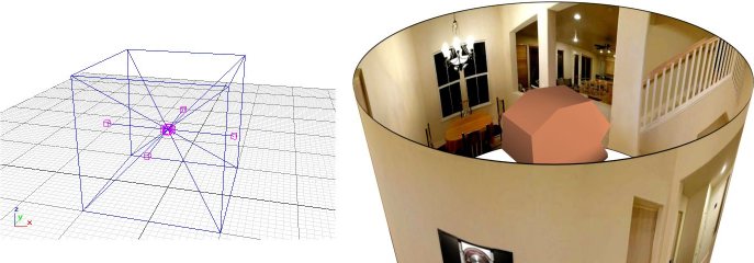
Figure 5: On the left: the four horizontal cameras in the listener's position make the "view cube". On the right: the listener's head and the view of his environment.

After separating the RGB components the columns are collapsed, to obtain three ring-like lists. (See Figure 6) This is corresponds to the reality, because the speakers are placed along a big ring on the same level.

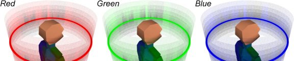
Figure 6: View of the listener's environment separated to RGB components (to three sound sources) where the columns are collapsed.

The length of the rings is equal to the sum of the columns of the images. The elements of rings contain the sum of pixel intensities in an image column. For example, if the resolution of the four horizontal images is 90 × 90, the size of each ring is 4 × 90 = 360. Moreover, each element contains the sum of the intensities of 90 pixels. Thus if 360 elements exist, then we can represent the sound intensity of a sound source at each degree in a one-dimension list. After this we have to normalize the list to [0..1] and weight for the channels of the speakers, from which the output waveforms can be generated. The output is predefined: 44.1 kHz, 16-bit, the number of channels is changeable.
    Let us first assume that the objects are still. The output file is built sample-by-sample, and is written in packages of the actual signal amplitudes of each channel. Each sample contains the weighted ring-value of the (maximum three) sound sources. The weighting (importance-function) depends on the position and the number of the speakers (Figure 1). Let us consider the generation of a single sample. We have a ring-list assigned to a sound source. Each element of the list is multiplied by the channel weight depending on the direction of the element, and the actual signal amplitude. These products are added for each speaker. These steps have to be repeated for each sound source (ring-list). Adding up these ring-results and writing out to its channels result in a package. Repeating these steps 44100 times, we get the output waveform that takes a single second.
    If the objects can also move, the ring-list can change in time. When the image refresh rate is 25 frame per second, the rings will be redefined at each 40 milliseconds. It means that if the sample rate of the sound is 44.1 kHz, then the rings are given new values at each 1764th sound sample. Between two frames an abrupt sound transition may occur. Avoiding this, we have to interpolate between two values of a ring. It is similar to as if we resample a 25 FPS film to 44100 FPS with linear interpolation. The only difference is that here the interpolation uses not the whole image, but only the rings containing the collapsed columns of the image.
    The basic advantage of the image based sound generation is that the size of objects in a perspective view is inversely proportional to the square of its distance from the listener (Equation 2). The sound intensity behaves exactly in the same way. Thus, scaling the loudness according to the image areas makes sense, because bigger viewable object surface means more intensive sound:

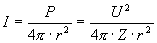
where I is the intensity of an omnidirectional sound source of P homogeneous sound power at distance r, U is the voltage amplitude and Z is the impedance of the system.
    The other advantage of the method is that no special image-synthesis algorithm is needed, because the used images can be rendered any existing rendering software (for example, Kinetix - 3D Studio MAX [5] [6] [7] [12]). Taking advantage of the similarity of sound and light spreading, this method handles the problems of area sound sources and partial occlusions. Using light dispersion we can model the sound dispersion. The disadvantage of the method is that it cannot handle the effects caused by speed of sound, including the Doppler effect, echo, phase shifting, etc. To simulate these effects, we also need the distance and the motion information of objects and the phase of sounds at any time, and not only at each 1764^th sample.
    In order to compute the distances, we can, for example, use one of the base colours (e.g. Blue). We place an point light source in the listener's position with distance depending intensity to get the distance information. The nearer objects are illuminated intensively and the further ones are dark. Thus the blue pixel intensities of the images are proportional to the distance. However, the object surfaces are usually shaded according to the illumination and shading models of computer graphics [1] [2], thus the visible colours will not be identical to the colour of the light source. Moreover, the distance information can be handled only in a single frame, but not between two frames. We do not have information about what happens between two frames. If an object is moving, its loudness is interpolated from the pixel information of the actual and the previous (or next) frames. For example, when a red object is moving from left to right, the red object on the left of the image becomes black in the next frame, because it moves to the right (volume fade out on the left). On the right side, the object turns gradually red from black (volume fade in on the right). This technique does not provide correct distance information, but it would rather generate something, which would mean that the red object moves away on the left and it approaches on the right in one frame time. The loudness simulates properly the movement, but the distance information is wrong. This can cause problems when we calculate the Doppler effect. The object on the left moves away with deep voice and it comes back on the right with a high-pitched tone. The problem of this method can be solved by some kind of shape recognition, which identifies the moving objects. The other disadvantage of this method is only one kind of distance (object-listener or object-light source) can be represented with the selected colour.
    If we want to use reflection(s), we have to consider all object distance types, including object-listener, object-object and object-light source. Thus we need a database (for example an ASCII Scene Export (.ASE) file from 3DS MAX or a VRML (.WRL) file [20]) that also stores the shape, extension, position, orientation and movement information. Such a complete database can be visualised by a special OpenGL [21] [22] program that renders the reference images. On these images we can identify the objects. Suppose that this time we do not use the collapsing operation and work directly with the 2D images. Finding the centre of mass of the projections of the identified objects, we can interpolate the centre and simulate the movement of the object. This is a working solution, but this is not free from problems either. One of them is how to calculate the centre of mass of the objects that surround us. The other one is how to handle the complicated objects having points with very different distances from the viewer.

5. Sound field computation using the 3D position and movement of each pixel

In this method we still work with 2D images and assume that the images are rendered in real-time. The method consists of the following steps. First it renders the images whose pixels contain the sound intensity information. The motion is analyzed by following the change of the pixel in which an object point is projected. Such a way, we can talk about the movement of pixels. Then the method assigns a record to each moving pixel, which contains the intensity of the pixel and two motion vectors which represent the 2D movement of the pixel from the previous and to the next frame, respectively. The record also contains the direct or indirect (reflected) distance of the sound source from the listener through the pixel. (See Figure 7)

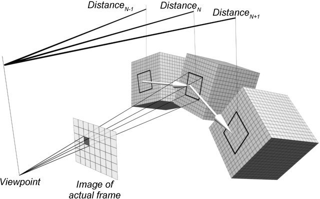
Figure 7: Calculating the record of a pixel. The cube in the middle is the sound source in the actual (N) frame, the left one is the same sound source in the previous (N-1) frame and the right one is the same sound source in the next (N+1) frame. The distances are direct distances and the two big white arrows are the motion vectors of the examined pixel.

The method calculates the record fields not only in the actual, but also in the previous and the next frames. The intensity of a moving pixel is set to zero in the previous and in the next frames. It is required, because in the neighbouring frames there is no guarantee that the examined pixel is visible or does not coincide with an another pixel. With this we make a fade-in and a fade-out effect. Summarising, each pixel of every image has the following record:

Table 1: Record of a pixel

	frame N-1 (prev.)	frame N (actual)	frame N+1 (next)
Intensity	0	Given	0
Distance	Calculated	Calculated	Calculated
Motion vector	Calculated	X	Calculated

The pixel intensities of the actual images are given. The distances and the motion vectors are calculated only by a 3D transformation. When we want to know the position of a pixel in the neighbouring frames (and the distance and the motion vectors from these positions), we have to determine the pixel's owner object and the position of the pixel in the coordinate system of its owner. This operation can be accomplished by inverting the viewing pipeline. The position and the orientation of the owner object determine the coordinates of the pixel, which move with its owner in the neighbour frames. From these coordinates we can calculate the remained record fields.

5.1 Generating the output sound waveform

The output waveform is generated like in the previous section, but here we also use a frame-time buffer. It means that each 40 ms waveform is generated in two parts. Let us examine how the algorithm works. After rendering the first image (without previous image) the algorithm calculates the record fields of each pixel by the data of the next frame. The next step is calculating the signal amplitude, phase shift and direction by an interpolation of record fields at each sound sample (one sound sample represents 1/44100 second). More precisely:
Firstly we need the waveform of the sound source and its timing (start and stop time). Then we get the length of soundwave-path (the distance between the sound source and the viewpoint through the actual pixel) from the pixel record. Using this distance with the speed of sound and the timing of soundsource we can calculate the phase shift of the sound wave. It is possible to calculate the absolute sampling phase of the waveform with the actual scene time (calculated from the frame rate, the number of actual frame and the time position between the actual and the neighbouring frames). This sound sample already contains the effects caused by sound propagation timing. The amplitude of the sound sample is defined by the intensity of the pixel. Motion vectors of the pixel determine the direction and weighting of sound sample. Finally these steps are repeated for each pixel.
Superposing the next frame's sound material that belongs to the current frame with the actual 40 ms sound material, we get the first 40 ms of the output waveform. (See Figure 8)

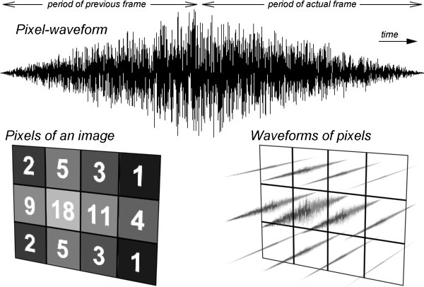
Figure 8: Calculating the waveform of a pixel.

6. Conclusions

This paper proposed several algorithms to compute the 3D sound field using rendering and image processing algorithms. The most sophisticated method uses the motion vectors of the pixels. The main advantage of this method over the method based just on the 2D images is that it also takes the movement of each pixel into account, thus it can handle the effects caused by the speed of sound (phase shift, Doppler effect, echo). Unfortunately, neither this method is really perfect, because in an unfortunate case interpolating, fading and superposing the sound of pixels can cause interference, which can distort the results. The other problem is the propagation of quantization error caused by too low amplitude (volume or loudness) of the added sound samples of the pixels. Using enough quantization levels we can avoid these errors and reach lower signal to noise ratio (SNR). The bigger quantization (bit depth) needs more operative memory. The database required by the motion vector method needs smaller storing space than the image lists used by image based approach. This database is specific, so the algorithm can handle limited input data formats, which cannot be interpreted some 3D modeller applications. Its other advantage is that its steps can be supported by the current graphics hardware. The 3D transformation of the pixels and the interpolation of the sound samples by frame and by pixel may slow down the computation. Choosing the right image resolution, we can find a reasonable compromise between production quality and the system requirements.

7. Acknowledgements

This work has been supported by the National Scientific Research Fund (OTKA ref. No.: T029135).

8. References

[1]    Dr. Szirmay-Kalos László (editor): Theory of three-dimensional computer graphics, Akadémia Kiadó, 1995.
[2]    Dr. Szirmay-Kalos László: Számítógépes grafika, ComputerBooks, 1999.
[3]    Barnabás Aszódi, Szabolcs Czuczor: Calculating 3D sound-field using 3D image synthesis and image processing, Képfeldolgozók és Alakfelismerők III. Konferenciája, 2002.
[4]    Füzi János: 3D grafika és animáció IBM PC-n, ComputerBooks, 1995.
[5]    Aurum-Boca: 3D Studio MAX, Aurum DTP Stúdió Kiadó, Kereskedelmi és Szolgáltató Kft., 1997.
[6]    Ted Boardman, Jeremy Hubbell: Inside 3D Studio MAX - volume II: Modeling and Materials, New Riders, 1998.
[7]    George Maestri, et al: Inside 3D Studio MAX - volume III: Animation, New Riders, 1998.
[8]    Juhász Mihály, Kiss Zoltán, Kuzmina Jekatyerina, Sölétormos Gábor, Dr. Tamás Péter, Tóth Bertalan: Delphi - út a jövőbe, ComputerBooks, 1998.
[9]    László József: Hangkártya programozása Pascal és Assembly nyelven, ComputerBooks, 1995.
[10]    László József: A VGA-kártya programozása Pascal és Assembly nyelven, ComputerBooks, 1996.
[11]    Dr. Budó Ágoston: Kísérleti fizika I. (mechanika, hangtan, hőtan), Nemzeti Tankönyvkiadó, 1970.

[12]    http://www.ktx.com (Kinetix Home Page)
[13]    http://www.goldwave.com (GoldWave Home Page)
[14]    http://www.dolby.com (Dolby Laboratories, Inc. Home Page)
[15]    http://www.wareing.dircon.co.uk/3daudio.htm (Audio and Three Dimensional Sound Links)
[16]    http://www.borg.com/~jglatt/tech/wave.htm (WAVE File Format)
[17]    http://www.soundblaster.com (Sound Blaster Home Page)
[18]    http://www.creative.com (Creative Tecnology Ltd. Home Page)
[19]    http://www.thx.com (Lucasfilm's THX Home Page)
[20]    http://www.vrml.org/Specifications/VRML97/index.html (The VRML Consortium Inc. Home Page)
[21]    http://www.sgi.com/Technology/OpenGL (Silicon Graphics Inc. Home Page)
[22]    http://nehe.gamedev.net (NeHe Productions Home Page)