|
Diffuse and specular interreflections with classical, deterministic ray tracing Gergely Vass gergely_vass@siggraph.org Dept. of Control Engineering and Information Technology
Abstract Today almost all the free as well as the commercial 3d graphics applications - which claim to be photorealistic - are capable to render images using the ray tracing algorithm. This method handles only one kind of light transport between surfaces, namely the total, mirror-like reflection. In this paper a simple practical method is going to be presented to extend the capabilities of the classical ray tracing algorithm. The proposed workflow makes diffuse light transport possible and the use of area lights instead of the common point, spot and directional lights. The possible difficulties applying the proposed procedure in different software environments is going to be discussed as well. Keywords: rendering, global illumination, ray tracing, reflectionThe great improvement in the computing power of standard desktop computers made possible to use complex rendering softwares to generate photorealistic images [5]. There are many commercial 3d graphics applications on the market, which simulate the behavior of light so convincingly, that the resulting image looks real. These programs use state of the art technology and are hard to get acces to. The widely used and the free 3d applications generate images in much less time, but use simpler rendering methods. These algorithms - like ray tracing - make lot of compromise in order to avoid long render times keeping the image as real as possible. In the next part these simple and commonly used rendering methods will be discussed focusing on their strengths and weaknesses.
Today's graphics systems are pixel based. This makes the basic step of image synthesis the calculation for each pixel's color. This color value is proportional to the incoming radiance to the camera from a given direction. This physical value is a very hard and resource intensive problem to solve for, even if the wave properties of light or the presence of liquids and gases are ignored. The problem can be expressed in the form of the rendering equation [6]:
This equation shows how the radiance (
Let us introduce the
Using the operator above the rendering equation can be written in a compact form:
The unknown radiance “L” is both dfgd inside and outside of the operator, which makes the problem very complex. Because the operator cannot be inverted it os not possible to eliminate the coupling. Fortunately the problem can be solved using a simple trick: the whole right side should be substituted in the unknown function of the same side. This transforms the integral equation into an infinite series:
The elements represent the direct emission, the single reflection, the secondary reflection and so on. The elements of the series are integrals with increasing dimensions. The simple rendering algorithms do not even try to solve the equation in this form. The local illumination method tries to solve for only the first two elements of the series, ray tracing eliminates the integral from every element making the series into a much simpler sum. Local Illumination Almost all of the commonly used 3d graphics programs make use of the local illumination model. This is a drastic simplification of the rendering equation. It is assumed that the look of real world surfaces can be determined by calculating direct emission and single reflection only. The rest of the infinite series is expressed in one, user defined ambient term. Using this assumption only one integral of one dimension should be calculated. This integral is supposed to sum the incoming radiance from all directions. Because this calculation is still hard and time consuming to do the local illumination model simplifies the equation even more. It is known that integrating any combination of Dirac delta functions is very easy, since the integral equals the sum of few values. In the case of the rendering equation the incoming radiance is a combination of Dirac delta functions only if the light sources are infinitesimally small. The local illumination model uses only ambient, directional, point and spotlights - and ignores objects with self illumination - when calculating the incoming radiance in order to eliminate the hard integral. This model would be useless if the generated pictures were far from real but fortunately that is not the case. In real life and especially in case of artificially lit environments the dominant light sources determine the look of objects, and the intersurface light reflections have only secondary importance. In cases when reflected light acts as important light source in the local illumination environment the user have to define more abstract lights to achieve the desired effect. This method is physically incorrect and it might be uncomfortable as well, however in production environment the method has proven it's usability [1]. The rendering equation using the local illumination model turns out to be very simple due to the Dirac delta type light sources:
Where the function Recursive Ray tracing The ray tracing algorithm [4] is a very common extension of the local illumination method. Using ray tracing the total reflection and the refraction of light can be simulated correctly. This effect is very important since the reflection seen on shiny surfaces - like chrome, glass or car paint - determine the overall look of these objects. The implementation of ray tracing is based on the local illumination model. Knowing the normal vector of the rendered surface element the reflection and refraction directions can be calculated. Calling the already implemented local illumination algorithm in these directions the value of the incoming light reflected or refracted toward the camera can be easily calculated. This process is able to work recursively and follow a “ray" from the camera along the path of the incoming light rays. This formula is the extension of the equation for local illumination (5). The two new terms are the reflected and refracted light rays which can be calculated recursively. If no abstract lights are used for the local illumination the only thing that effects the final rendering is the self illumination and ray tracing:
This equation is practically equation (6) without the terms of equation (5). If only non-transparent surfaces are used the third term can be ignored. Considering the first two terms it is surprisingly similar to the rendering equation in the form of equation (3). The recursive ray tracing algorithm doesn't neglect any term of the infinite series, the only simplification comparing to the original is the BRDF which consists of Dirac impulses. This likeliness makes the use of the ray tracing method possible to calculate the rendering equation, or in other words: to solve global illumination problems. Global Illumination There are numerous methods to solve the rendering equation [6] with no - or not much - simplification. These algorithms - like Monte Carlo integration [8] - often handle not only mirror like surfaces but glossy and diffuse objects as well and are called global illumination renderers. The goal is to achieve the same realistic result with the commonly used ray tracing softwares without the need of modifying the program.
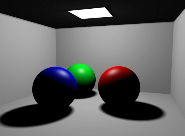
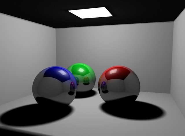
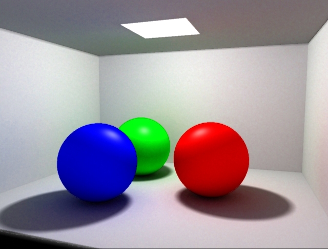
Figure 1. Images generated using local illumination, ray tracing and global illumination methods.
There are some tricks used in the 3d graphics community intended to simulate the effect of global illumination. These tricks - often called “fake radiosity" methods - can be classified into two major groups:
The proposed method works for all objects in the scene and is far more physically accurate than the available “fake radiosity" tricks. The main goal is to prepare the ray tracing algorithm to handle glossy and diffuse reflecion. The local illumination capability of the softwares is not used at all, since it doesn't calculates any secondary light reflection. However, local illumination – using models like Phong and Lambert – could be used to calculate the “first shoot” or the direct illumination of lights but this option was thrown away because the following reason. It required to have point lights defined – instead of light emitting objects – thus the characteristic shadows would be not soft at all. In fact the local illumination method is not able to generate realistic soft shadows, which is overcomed using ray tracing for the first shoot too.
It has to be investigated how diffuse materials work in the real world to achieve the same result on the virtual surfaces. The perfectly diffuse behavior is described by the Lambert model. This model supposes that the incoming light is reflected in all directions with the same intensity. In reality diffuse objects have such microscopic structure that the incoming rays are reflected to all direction independently from the incoming direction. The algorithms which use the microfacet model [2,9] simulate this effect with little, randomly oriented micromirrors called facets. This idea is very useful to create diffuse or glossy materials while rendering with ray tracing. The 3D programs offer usually 3 alternative ways do define the geometry or the structure of the surface [11]. One way should be chosen to create these random displacements in order to create diffuse surfaces. Microstructure: Using the local illumination model an empirical BRDF - like Phong or Lambert model – is assigned to every surface. This means that the light reflection properties of some material due to the microscopic and atomic structure are simulated by abstract mathematical formulas. During ray tracing these illumination models are unimportant in determining the reflection and refraction directions, thus these formulas will not be used.
Macrostructure: The structure of diffuse and glossy surfaces can be modeled using standard and widespread surface modeling methods. Either NURBS, polygon or subdivision surfaces could be used to describe the geometry of the surface. However, this approach requires lot of memory - way more than an average user has - to store even a very simple and rough estimation of some diffuse surface.
Mesostructure: To model the visible roughness of a surface bump maps are used. These require very little memory - especially when using procedural textures - and are able to change the reflection and refraction directions during ray tracing. The main idea of bump maps is that using the partial derivatives of a standard texture the normal vector of the surface can be perturbed. This creates the impression in the viewer as if there were bumps on the surface. It is the ideal for us to choose this approach since it is supported in all 3d graphics packages, it is fast and requires almost no memory.
The only thing that affects the light reflection properties of the materials is the bump map. The goal is to create surfaces that can reflect light in every possible direction. To make a diffuse material based on the Lambert rule it is necessary that the probability density of the direction of the reflected ray to be constant. This means the bump map “rotates” the normal vector in any direction with the same probability. If the bump is smoother more rays will be reflected towards the ideal reflection direction and the material will look glossy. To achieve this effect a very dense, high frequency bump map should be used since the user does not want to see the actual microscopic structure of the material. However, there are lots of materials in real life which do not work this way. Satin, velvet and dense hair have such microscopic structure that the majority of the reflected rays point not toward the ideal reflection. These non-isotropic structures [2] can be modeled with such bump maps that reproduce the effect of microscopic features shadowing certain directions or reflecting light to another specific direction. The first attempt to define the bump map was to generate textures that would represent a user given normal vector distribution. This approach has had seriuos disadvantages:
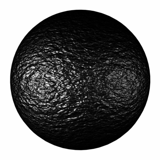
The next approach was to perturb the normal vector with a custom script. This would not work, however, because even the most advanced 3D applications are not prepared to give this option to the user. The way of generating bump maps in the research turned out to be using built in textures. These textures generate noisy displacements with no visible repetitions. Modifying the gain of the texture the depth of the bumps could be changed, thus the light reflection properties of the material also changed. By modifying the texture parameters and rendering test pictures the diffuse or glossy behavior could be achieved.
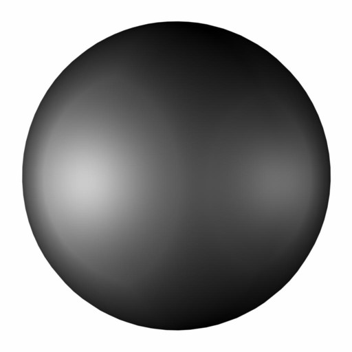
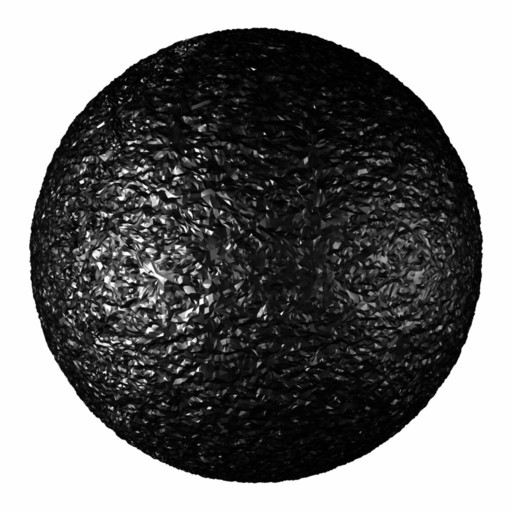
Figure 5: Using the same texture with different gain to generate the bump map.
Using the ray tracing rendering method to define the picture, the program shoots rays from each pixel to hit a surface. If an object is hit - and no local illumination is used – the color of the current surface element is calculated using equation (7). Since this process is a recursive one the rays from the camera do not stop at the first intersection but follow certain paths along the reflections. These paths will be used – certainly more for each pixel – to calculate the color of the pixel defined by the rendering equation (1).
As stated above the rays shot from the camera follow a path or gathering walk since they are reflected at each surface collecting the incoming radiance. Every time one of these rays hits a surface the “collected” light is the sum of the self illumination and the light from the reflection. There might be two kind of dangerous situations while rendering:
Apparently one ray shot from each pixel is not enough. To understand why many gathering walks should be started from each pixel the common integral formula should be investigated. This is useful since the goal is to calculate the integral of equation (1).
where n is the number of samples, s() is the weight function and
where n is the number of samples for each pixel and The main question is: what n should be used to achieve good quality? There is no global answer since the amount of noise seen on the picture and rendering time is in direct proportion to the number of samples.
Figure 6: The same scene rendered using 1,3,10,32 and 320 samples for each pixel
The 3D application used [7,10] for the tests let the number of samples to be 32 at maximum which turned out to be not enough. To overcome this limitation more images should be rendered from the same scene. If the renderer uses stochastic sampling – and the random generator uses different seeds for each frame - the starting points of the gathering walks will be at slightly different position. Averaging these pictures the result will be as if more samples were used for each pixel. Apparently the user should not rely on the renderer this much since the same result can be achieved using only one sample for each pixel even if the sampling positions are static. The trick is to animate the position of the bump texture. Doing this the reflection directions will obviously change since bump map changed while the probability density of the reflection direction will fortunately not be affected. The images rendered this way can be averaged together producing the same image as if it was rendered with a very high number of samples. Using the proposed method global illumination problems can be solved without any major simplification using standard 3D packages with ray tracing capabilities. The user can define light emitting objects instead of abstract point light thus generating realistic soft shadows. The specular and diffuse interreflections can be simulated as well not like while using the renderer the conventional way. The application of the method does not require any special training or programming knowledge, any standard – even freeware – renderers can be used. Unfortunately the generation takes long and the final pictures contain significant noise. To reduce this artifact the number of samples should be extremely increased causing the computer to render even longer. This noise makes for most of the cases impossible to use the pictures without any modification or filtering. However, there are many ways to make use of this process in production environment. The generated pictures are great visual references for the technical directors how to lit their scenes using local illumination. It is also useful to filter out the high frequency noise and use the generated pictures as textures for the objects in the scene. The subject of future investigation might be the efficient reduction of the noise with some custom filter or other method. The generation of any microfacet structure would be also useful to render non-isotropic objects.
This work has been supported by the National Scientific Research Fund (OTKA ref. No.:T029135). The test scene with the car has been modelled and rendered by Maya, that was generously donated by Alias|Wavefront.
[1] Apodaca, T., Gritz, L.: Advanced Renderman – Creating CG for Motion Picture (chapter 1.), Morgan Kaufmann, 2000. [2] Ashikhmin, M., Premoze, S., Shirley, P.: A microfacet-based BRDF generator, in Proceedings of SIGGRAPH 2000, p. 65-74 [3] Campin, E.: Faking radiosity in Maya (tutorial), www.pixho.com [4] Glassner, A.: An Introduction to Ray Tracing, Academic Press New York, 1989. [5] Greenberg, D., Torrance, K., Shirley, P., Arvo, J., Ferwerda, J., Pattanaik, S., Lafortune, E., Walter, B., Foo, S., Trumbore, B.: A framework for realistic image synthesis, in Proceedings of SIGGRAPH 97, p. 477-494 [6] Kajiya, J. T.: The rendering equation, in Proceedings of SIGGRAPH 86, p. 143-150 [7] Pearce, A., Sung, K.: Maya software rendering – a technical overview, Alias|Wavefront, 1998, www.aw.sgi.com [8] Szirmay-Kalos, L.: Monte-Carlo Methods in Global Illumination, http://www.iit.bme.hu/~szirmay/script.pdf [9] Szirmay-Kalos, L., Kelemen, Cs.: A microfacet based coupled specular-matte BRDF model with importance sampling, Eurographics Conference, 2001, Short presentations, pp 25-34. [10] Woo, A.: Aliasing artifacts in Maya – a technical overview, Alias|Wavefront, 1998, www.aw.sgi.com [11] Yu, Y.: Image-Based Surface Details (introduction), Course 16 in Course Notes of SIGGRAPH 2000, p. 1-1.
|
 (1)
(1) ) can be calculated from a given surface element: the surface's light emission (
 ) and the fraction of the incoming light that reflects to the camera should be added together. In order to express the second term the light from all possible incoming direction should be taken into account weighted with the bidirectional reflectance distribution function (BRDF) and the cosine of the incoming angle.
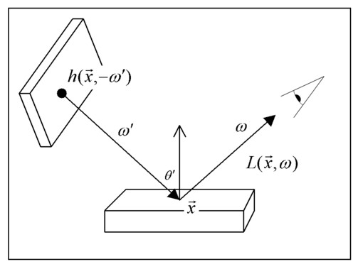
 integral operator, which describes the light-surface interaction:
 (2)
(2) (3)
(3) (4)
(4) (5)
(5) represents the the incoming radiance from the i-th lightsource to the point
  from the direction
  . In this equation the rendering equation (1) is reduced to the sum of few, easily computable terms.
 (6)
(6) (7)
(7)
 (8)
(8) are the sampling points. In the actual case the radiance value given by the rendering equation should be estimated for each surface element hit with a ray. This means the samples will be the values of reflected light rays in different directions. The more rays are shot from the pixels the more accurate the result will be. If a bump map defining glossy reflection is applied more rays – samples – will be reflected toward the direction of the ideal reflection. If the bump defines a diffuse material all samples will have probably different direction. No gathering walk is more important than the other, thus no weight function is used:
  (9)
(9) is the reflection direction of the i-th ray. In this equation the refraction is ignored.