Milos Hasan
milos.hasan@inmail.sk
http://frep.miesto.sk/
Faculty of Mathematics, Physics and Informatics
Comenius University
Bratislava / Slovakia
In the past, implicit surfaces have been recieving less attention in
modeling software than parametric surfaces like Bezier and NURBS patches. Why is this so? The basic advantage of the parametric paradigm is contained in the following example: It is much more straightforward to draw a circle using (cos(t), sin(t)) than with x2+y2=1. Moving from curves to 3D surfaces, a parametric description of a surface in the form
|
|
If no particular restrictions are put upon the defining function f of the implicit surface, then a large number of operations is possible: set-theoretic operations, blending and morphing the surfaces, space deformations, sweeping, and others. Doing these with parametric surfaces would be nearly impossible. However, if nothing is known about the function f except an evaluation algorithm, both polygonization and ray tracing are quite slow, have numerical problems and are tedious to implement. On the other hand, ray tracing really benefits from a restricted choice of the function f - if it is a quadratic polynomial in x, y, and z, then f(g(t)) is a quadratic function in t, with a well-known closed form solution. Of course, the range of possible shapes of quadratic surfaces is too limited. This paper tries to investigate what is between these two extremal cases, hoping to find ''classes'' of functions which allow for better visualization algorithms while preserving enough shape variety. These classes differ in the structure of the algebraic expression that defines the function f.
The rest of the paper is structured as follows: The next section contains the definition of functional representation and an overview of the rich set of operations it allows for. Theoretical development of the notion of a ''function class'' is presented in section 3. The language HyperFun and its translation into a target function class is discussed in section 4. Section 5 contains several examples of possible usage of the theory.
Many different kinds of implicit surfaces were invented by various researchers, but the concept of function(al) representation, proposed by Pasko et al [1], serves well as a unifying idea:
Definition 1
Consider the continuous function f:Rn ® R and the geometric object G in Rn defined as:
The function f will be called the defining function of G, and the inequality f(x) ł 0 will be called the functional representation (F-rep) of G. Discontinuous functions can be used too, by taking the closure of the resulting point set.
G={x Î Rn|f(x) ł 0}
These are defined by polynomials in several (usually three) variables. First degree (linear) polynomials define planes, or more exactly half-spaces. Second degree polynomials, often called quadrics, can define spheres, ellipsoids, cones, cylinders, etc. A torus is an example of a 4th degree surface.
Constructive solid geometry (CSG) [4] is a way to combine any implicitly defined objects into a tree by set-theoretic operations like intersections, unions and differences. Ray tracing of the tree is straightforward, if we know the ray intersections with the functions in the leaves. Interestingly enough, the functions defining the input objects can be combined into a new function in the following way:
This was proposed by Ricci in [2]. Another formulation by Rvachev [10]:
The R-functions are often favored over the min/max functions for set-theoretic operations, because of their C1 continuity everywhere except (0,0), which is especially useful for blending and morphing. However, the min/max solution leads to less complicated expressions.
A space deformation, or bijective mapping, is a function f:Rn® Rn. Deforming an object defined by the function f yields f(f-1(x1,...,xn)). A typical example is an affine transform (rotation, scaling, ...).
Blending is similar to set-theoretic operations, except that it produces smooth transitions instead of sharp edges. One of the many possible solutions can be found in [1]:
The parameters a, b, and c control the final shape.
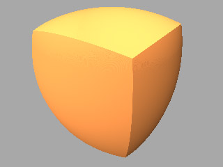
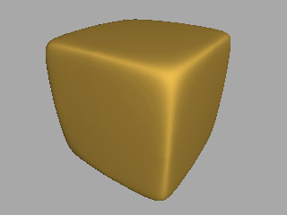
Morphing with F-rep is really easy - it is just a linear combination of the defining functions. If we want an object that is one third of a sphere and two thirds of a cube, we define:
|
Blinn [9] proposed to define an implicit function as a sum of several ''field functions'' of the form
|
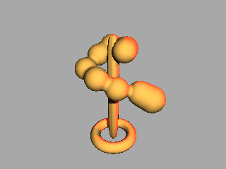
HyperFun [5] is a simple special language for defining F-rep objects. It is similar to C or Pascal, but only allows for real numbers. An example from the tutorial at www.hyperfun.org:
--This HyperFun program consists of one object:
--union of superellipsoid, torus and soft object

my_model(x[3], a[1])
{
array x0[9], y0[9], z0[9], d[9], center[3];
x1=x[1];
x2=x[2];
x3=x[3];

-- superellipsoid by formula
superEll = 1-(x1/0.8)^4-(x2/10)^4-(x3/0.8)^4;

-- torus by library function
center = [0, -9, 0];
torus = hfTorusY(x,center,3.5,1);

-- soft object
x0 = [2.,1.4, -1.4, -3, -3, 0, 2.5, 5., 6.5];
y0 = [8, 8, 8, 6.5, 5, 4.5, 3, 2, 1];
z0 = [0, -1.4,-1.4, 0, 3, 4, 2.5, 0, -1];
d = [2.5, 2.5, 2.5, 2.5, 2.5, 2.5, 2.5, 2.7, 3];
sum = 0.;
i = 1;
while (i<10) loop
     xt = x[1] - x0[i];
     yt = x[2] - y0[i];
     zt = x[3] - z0[i];
     r = sqrt(xt*xt+yt*yt+zt*zt);
     if (r <= d[i]) then
          r2 = r*r; r4 = r2*r2; r6 = r4*r2;
          d2 = d[i]^2; d4 = d2*d2; d6 = d4*d2;
          sum = sum + (1 - 22*r2/(9*d2) + 17*r4/(9*d4) - 4*r6/(9*d6));
     endif;
     i = i+1;
endloop;
soft = sum - 0.2;

-- final model as set-theoretic union
my_model = superEll | torus | soft;
}
It is important to remember that the notions of ''object'' and ''function'' are often freely interchanged, although a single object can have infinitely many defining functions. In the following, classes (sets) of functions will be discussed, as opposed to the sets of objects definable by those functions.
These operations will also be used in the text:
The D operation always creates a continuous function, if the input functions are continuous. This is not the case with the if operation. D(f,g,h) and if(f,g,h) can be very different functions, but they define the same object.
Definition 2
The class F of continuous functions on Rn will be called a primitive class, if it satisfies the following:
f(xo+txd)=g(t) ł 0
Definition 3
Consider a class F (not necessarily primitive) and operations o1,Ľ,ok. The class of functions generated from F by these operations, i.e. the smallest class containing F and closed under o1,Ľ,ok will be denoted by F(o1,...,ok).
Theorem 1
F(min, max) and F(if) are closed under linear combination for any primitive class F.
F(D) = F(min, max) Í F(if) = F(min, max, if)
Note that while the classes F(min, max) and F(if) are different, the classes of geometric objects with defining functions from them are always the same, because replacing all if's by D's does no change to the object. So it does not really matter which class we use. The previous ideas can be formalised in the following way:
Definition 4
Suppose the sets of objects definable in classes of functions F and G are the same (and the two representations can be algorithmically converted between each other). This fact will be denoted as F ~ G - F and G are similar.
F(min, max) ~ F(if)
From now on, the process will continue as follows: Take a HyperFun program and try to extract the function it defines (as an algebraic expression). Choose a target function class and try to apply transformations to the algebraic expression in order to get an expression in that particular class. The transformations should do as little change to the underlying geometric object as possible. If the transformation turns out to be impossible, the ''difficult'' parts of the object have to be left alone and rendered numerically or just skipped.
The current problem is as follows: the input is a HyperFun program (a syntactic object) and the output should be a function that it computes (an expression, a mathematical object). The very last function in the HyperFun program is the actual defining function of the model. So, the procedure basically consists of carrying out a symbolic computation of the term f(x, y, z, c1,Ľ,ck), where f is the last function in the program, x, y, z are symbolic names of variables and c1,Ľ,ck are actual constants. During the process of the symbolic computation, the following structures can occur:
By now, the algorithm created a complicated expression containing the symbolic variables x, y, z, constants, and applications of arithmetic operations, minimum, maximum and if functions, and other mathematical functions over the variables and constants. The next step is to apply different replacement rules onto the expression, in order to get it closer to our target class (e.g P(min, max)). The replacement rules fall into three cathegories:
|
|
The best way is to apply the rules in this order: first function-invariant rules, then object-invariant rules, then approximation rules. This, for example, guarantees correct display of the if-then-else statements in the HyperFun program. If the if functions were converted to D functions right away, the object could come out different than expected.
|
The function classes P(min, max) and P(if) and the corresponding object class P* seem to be very useful - besides set-theoretic operations and affine transforms, they are closed under some other non-obvious operations.
It was shown before that F(min, max) is closed under linear combination for any primitive class F, and morphing is basically a linear combination of defining functions. Let's look at an example of a HyperFun program that describes an intermediate object between a sphere and a cube, like in section 2.5.
morph(x[3], a[1])
{
    sphere = 1 - x[1]^2 - x[2]^2 - x[3]^2;
    cube = x[1]+1 & 1-x[1] & x[2]+1 & 1-x[2] & x[3]+1 & 1-x[3];
    morph = 0.75*cube + 0.25*sphere;
}
In the first step, the program will be translated into
|
| min(-0.25*x2 + 0.75*x - 0.25*y2 - 0.25*z2 + 1, |
| -0.25*x2 - 0.75*x - 0.25*y2 - 0.25*z2 + 1, |
| -0.25*x2 - 0.25*y2 - 0.25*z2 + 0.75*y + 1, |
| -0.25*x2 - 0.25*y2 - 0.25*z2 - 0.75*y + 1, |
| -0.25*x2 - 0.25*y2 - 0.25*z2 + 0.75*z + 1, |
| -0.25*x2 - 0.25*y2 - 0.25*z2 - 0.75*z + 1) |
Because of the decision to use min and max instead of R-functions for Boolean operations, the standard F-rep blending unions and intersections with offset functions are impossible. However, there are other options - because of the fact that any blending operator is itself a 2D function, it is possible to build a suitable one via 2D F-rep.
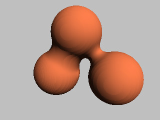
Note that one of the two branches of the xy=1 hyperbola looks like a promising blending function, which leads to the following definition of blending:
Parameter a controls the amount of subtracted/added material. The functions can be easily extended to support multiple blend:
Of course, the multiplication in the last argument raises the degree of objects: the resulting object's degree is generally the sum of the degrees of the input objects. The blended cube shown on the picture is therefore a P3* object.
There are other possibilities to ''cut'' the second branch of the hyperbola, but they are harder to extend to multiple blends.
A well-known 6th-degree polynomial field function f(r) was proposed by Wyvill in [6], with the properties:
|
|
The problem is that the resulting expression grows exponentially with the number of summed field functions. However, there is a solution: a special algorithm for raytracing soft objects, convolution surfaces and some other surfaces was proposed by Sherstyuk in [3]. So let's denote as C the primitive class of functions allowed by this algorithm and use (PČC)(min, max) as the target class.
This paper outlines a new approach to implicit (F-rep) modeling. Geometric objects are defined by algebraic expressions with a restricted structure, which allows for faster rendering (especially ray tracing) algorithms. It combines modeling in the HyperFun language (which is suitable for the user) with a CSG-like representation (which in turn suits the ray tracing algorithm better).
I am already working on the implementation of the HyperFun parsing and conversion algorithm, which should produce an intermediate representation of the object, suitable for input into a CSG raytracer.