5 Experiments and Results

All versions of the algorithm from section 3 were implemented in Borland Delphi 5.0. It has been tested on 25 models from data sets from [9,10,2]. Experiments have been performed on a PC AMD Duron 850MHz with 256MB of RAM and Geforce 2 MX graphic card, running on MS Windows 2000 system. The implementation was compared to one of the best known publicly available algorithm - STRIPE (http://www.cs.sunysb.edu/~stripe/) with default settings. The times of I/O operations have been excluded from measurements.

Tables 1 and 2 show comparison of the classic OpenGL rendering method, extensions, triangle strips and triangle strips combined with extensions. Table 1 shows the frame rate and Table 2 shows the ratio of tested method frame rate to classic method frame rate. To be able to make one triangle strip per mesh even for large data sets, we decided to use artificial data (i.e., planar rectangular grid). In these two tables we want to show the advantage of using triangle strips and OpenGL extensions.

 

 

Table 1: Frame rate - comparison of classic calls, extensions, triangle strips and extensions + triangle strips. All values are in frames per second.

 

 

Table 2: Ratio - comparison of classic calls, extensions, triangle strips and extensions + triangle strips. Values are computed relatively to the classic method.

Extension speedup is close to theoretical bounds (about 1.85 for larger data sets). The difference is probably caused by the border of the grid, where the vertices are used only three times. The speedup while using triangle strip is a bit smaller (about 2.7 for larger data sets) than expected. This difference could be caused by the swaps that are needed to cover the grid. While using the combination of both methods, the speedup is close to the theoretical expectation (strips speedup * extension speedup). This measurement also affirms the theory that the speed is not bounded by the rendering process itself but by the rate at which the data are transmitted into the graphical processor.

Table 3 shows the information about data sets used in tests presented below. We have chosen eleven models that are often used in other papers and are available.

 

 

Table 3: Set of testing models.

Next tables show a comparison of the SGI based method with all four modifications and the STRIPE algorithm. Table 4 shows the number of strips in the models. For bigger models, the behavior of all modifications of SGI is the same as we expected. RN method is the worst one and LNLN gives the best results. Except the ellipsoid (3), STRIPE is worse than the SGI LNLN method. For bigger data the STRIPE algorithm was too slow and we got incorrect output (the same behavior as reported e.g. in [11]).

 

 

Table 4: The number of strips needed for model.

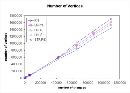
In Table 5, the number of vertices after stripification is shown (for graphic interpretation see Fig. 3). The LNLS method is better than the original method. STRIPE algorithm is worse than LNLN and LNLS method (except ellipsoid (3)).

 

 

Table 5: The number of vertices needed for model.

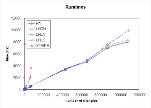
The comparison of time is presented in Table 6 (for graphic interpretation see Fig. 4). Although the condition in RN method is short, the time is worse than the other methods. This is probably caused by bigger number of strips and bigger number of vertices which increase the number of other decisions. The fastest is method LNRN. The STRIPE algorithm seems to be very slow (four and more times slower than any other method).

 

 

Table 6: Time needed for stripification in milliseconds.

One of the reasons why the STRIPE seems to be so bad is that STRIPE is constructed for data sets that are not fully triangulized, but our testing models are fully triangulized. This is a bit unfair, because only the local algorithm is used. The reason why we decided to use STRIPE as a testing method is that many other authors use it and so we are able to compare our method to them indirectly. We do not know why the STRIPE fails on bigger data, but it is not only our experience. The same behaviour is mentioned also in other papers ([11,3] and even the authors of STRIPE [6] are testing the algorithm on small data only). We briefly checked the code of STRIPE and we found some non-optimal parts of code that slow STRIPE down.

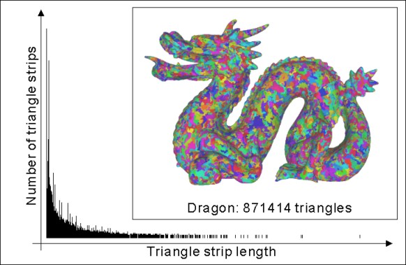
We have also tested the length of strips. The typical histogram obtained by LNLN method is shown on Fig. 5 (dragon). As you can see, in a typical model most of the strips is quite short but there exists a limited number of strips that are much longer. We have tried to normalize the histogram by cutting the long strips to avoid breaking the triangulation, but the effect was different than we expected: both the number of triangles and the number of vertices increased as we have decreased the maximum length of a strip.

From these results, a conclusion can be done that from SGI-based method, LNLN provides the smallest number of strips while LNLS needs the smallest number of vertices. The difference in rendering time while using a model stripified by LNLN and LNLS method is less than 1%. RN and LNRN modification provided slightly worse results. The STRIPE algorithm gave relatively bad results although it is widely used as a comparative standard in stripification papers.

  

Figure 3: Number of Vertices.

  

Figure 4: Runtimes.

  

Figure 5: Typical histogram of length of strips using LNLN method. The Dragon model has 17401 strips.