Keywords: Point cloud, Morphing, Clustering
The representation of geometric models by large sets of point samples (a.k.a point clouds) constitute one of the canonical data formats for scientific data visualization. We can acquire point clouds from the measurement of some physical process. Point clouds can represent surfaces, volumetric or iso-surface data. The availability of the modern 3D scanners brings the possibility to acquire point sets representing the surface of the analyzed solid, that contain millions of sample points.
Point cloud can be for some applications better representation than widely used boundary representation. This holds mainly for very complex models, such as fractal surfaces. It is generally good idea to store these object as point clouds, because the algorithms for conversion to the surface representation (such as polygonal mesh) are very computationally involved and require great amounts of main memory. One reason for the inefficiency of boundary representation is that highly detailed models contain a large number of small primitives, which fill lesser area than a pixel when they are projected and displayed.
Point cloud is the unstructured set of point samples. One point sample is elementary object, specified by its location in 3D space, normal vector, color, transparency and size. Single point sample can be visualized as a small sphere or a point (pixel). As presented in [2], [4] and [5], a point set representing the surface of a model can be rendered as a solid textured surface.
The morphing between two solids is the animation, during which the solid smoothly changes its shape from one shape to another. Our goal is implement and analyze several methods, which may be theoretically applicable to morphing between two point clouds. The methods should be independent of the topology of the models (should consider only the locations, possibly normals of the point samples) and should be able to perform morphing between two different-sized point clouds.
The fundamental principle underlying all introduced methods is the finding of the mapping
 S and di
D, di
=
S and di
D, di
=  (si). In
reality the situation is slightly more
difficult, because one point
of the source set can be assigned to multiple
points of the destination set and vice-versa. Therefore
the morphing can be expressed
by the set of point couples
M = {(si, di) | si
S, di
D}. The
morphing can be performed by
the computing of the location of the points pi of
transition solid, pi = f(si, di, t), where t
<0, 1> is the
progress of morphing. If we choose the
straight motion paths, the function f will
be simple linear interpolation. The resulting number of points involved in
morphing is equal to the cardinality of the set M.
Therefore the whole problem with morphing can be reduced to the finding of
the suitable relation
.
(si). In
reality the situation is slightly more
difficult, because one point
of the source set can be assigned to multiple
points of the destination set and vice-versa. Therefore
the morphing can be expressed
by the set of point couples
M = {(si, di) | si
S, di
D}. The
morphing can be performed by
the computing of the location of the points pi of
transition solid, pi = f(si, di, t), where t
<0, 1> is the
progress of morphing. If we choose the
straight motion paths, the function f will
be simple linear interpolation. The resulting number of points involved in
morphing is equal to the cardinality of the set M.
Therefore the whole problem with morphing can be reduced to the finding of
the suitable relation
.
The assignment process can be based on various criteria. Probably the most commonly used criterion will be that the total distance, which the individual points travel during the morphing, is minimal. In this case the finding of mapping M is equivalent to the solving of the optimization problem
 (si, di) is the real-valued
nonnegative metric function. In the simplest
case, where the paths between source and destination points are lines, the
Euclidean distance between source and destination points is the appropriate
candidate for the metric
(si, di).
The metric can depend also on the additional attributes of point samples,
such as the orientation of both normal vectors.
(si, di) is the real-valued
nonnegative metric function. In the simplest
case, where the paths between source and destination points are lines, the
Euclidean distance between source and destination points is the appropriate
candidate for the metric
(si, di).
The metric can depend also on the additional attributes of point samples,
such as the orientation of both normal vectors.
The trivial algorithm, which finds all possible assignments and chooses the optimal solution based on the optimization criterion, is unusable because of its exponential computational complexity. Where this algorithm can be used for finding the assignment between small point sets (max. 10 points), the models represented by point cloud contain thousands, possibly millions of sample points. We can find the assignment by incorporating the algorithms of artificial intelligence (searching in the state space), genetic algorithms, or space partitioning (clustering). This report introduces several methods based on clustering.
The idea of clustering is to group the points into a smaller number of clusters and find the mapping M between the two sets of clusters. The motivation behind the use of clustering is basically to reduce the problem size, solve the morphing on the higher level (cluster level) and then descend to the lower level. This approach is based on “divide and conquer” programming technique.
Clustering is one of generally used methods for the simplification of the point-sampled geometry. In the process of clustering the unstructured point cloud is divided to several smaller, spatially compact subsets (clusters). The clusters can be in the next step of simplification replaced by single point samples, whose size will reflect the size of replaced cluster. Two methods of clustering are clustering by incremental region-growing and hierarchical clustering. In our implementation we will use the latter method. This method is suitable for our needs, because it organizes the point cloud by creating the hierarchy of the subsets of point cloud. All implemented methods are based on the methods for efficient point cloud simplification from [1].
The hierarchical clustering is based on the partitioning of the point cloud. The recursive algorithm divides the point cloud P to several smaller point clouds (clusters). The result of the algorithm is tree, whose nodes represent point sets. The root represents the point cloud P, the leaves represent the terminal clusters (which are further indivisible and whose size is smaller than the specified limit or which contain only one point). The presented algorithms will be shown on the hierarchical clustering using binary space division (BSP tree). Other similar data structures, such as octrees, can be also used [4].
The hierarchical clustering using binary partition performs recursive division of point cloud to two parts by the split plane. The split plane is determined in most cases by the anchor point (usually the center point - centroid of the point set) and the normal vector. The choice of normal of the split plane has great impact on the quality of the morphing. The division algorithm is then applied to two resulting point sets. The cluster is divided only if its size is larger than the specified limit. In the text below, several possible methods for the finding of the normal of splitting plane are shown. As the anchor point of the splitting plane we will choose in most cases the centroid of the point set. For the covariance analysis is the centroid the only plausible choice; for the other methods we could use also other points, such as the center of bounding box/bounding sphere of the point set.
In this straightforward algorithm the normal of split plane is chosen alternately in the direction of x, y and z axis, depending on the depth of divided cluster in the binary tree (see figures 1 and 2).
|
|
This method is very easy to implement. The disadvantage of this method is that the point cloud is split by orthogonal cuts, which can be visible during the morphing. For the reduction of this undesirable phenomenon we can apply a random noise function to the normal vector of the split plane.
This method is based on the division of the (axes-aligned) bounding box of the point cloud. The parameters of the bounding box are computed from the coordinates of all point samples and the bounding box is split into two equal halves by the plane perpendicular to its longest axis. This method does not necessarily involve the computation of the centroid for each cluster (the anchor point for the splitting plane can be chosen as the center of the bounding box), but we must find the dimensions and location of the bounding box. The bounding box can be specified by two points in 3D space, representing the lower front left and upper back right corners. This method leads to decent results, compared to orthogonal clustering. However, the method is more computationally expensive than the former method, since the finding of the corners of the bounding box takes several times (roughly twice) more time than the finding of the centroid.
The normal vector of the split plane can be found using the covariance analysis of the neighborhood of the centroid of the point cloud. The covariance analysis allows us to estimate various local surface properties, such as normal vector of approximation surface or surface variation. The covariance matrix C of the point cluster P is defined as
 i, i
{0, 1, 2} are real-valued and
the eigenvectors vi, i
{0, 1, 2} form an orthogonal
basis. The eigenvalues
i measure the
variation of point set along the direction of the corresponding eigenvector.
i, i
{0, 1, 2} are real-valued and
the eigenvectors vi, i
{0, 1, 2} form an orthogonal
basis. The eigenvalues
i measure the
variation of point set along the direction of the corresponding eigenvector.
If we assume that
0 <
1 <
2, the plane
 0 expresses in this particular
case the variation of the surface
along the normal v0,
or by other words it estimates
how much the points of surface deviate
from the tangent plane. For more detailed description see
[1].
0 expresses in this particular
case the variation of the surface
along the normal v0,
or by other words it estimates
how much the points of surface deviate
from the tangent plane. For more detailed description see
[1].
The normal vector of the split plane will be defined by the centroid of P and the largest eigenvector of the covariance matrix of P (which is v2). The point cloud is always split along the direction of greatest variation, see the figure 3.
|
The drawback of this method is increased computational complexity (although the asymptotic complexity remains the same). Besides the centroid we must evaluate the coefficients of covariance matrix C (since the matrix is symmetric, there are six coefficients), find the roots of characteristic polynomial of C and finally compute the eigenvector corresponding to the largest eigenvalue.
The trees Ts and Td created by the clustering of starting and final point-cloud model in the next stage serve as input for the algorithm for the generation of assignments M = {(si, di)}. The algorithm is pretty straightforward: in each step will be assigned one cluster from Ts to some cluster from Td. In the beginning the roots of both trees are assigned one to another and the assignment is put to the ordinary queue. In the next step, the assignment (cs , cd) is extracted from the queue. If any of the clusters cs, cd is a leaf, the assignment is put again to the queue, else the children of cs and cd are examined, assigned to each other and these assignments are put to the queue. This step is repeated until the queue contains only the assignments of type (cs, cd), where at least one of cs or cd represents a leaf in the corresponding tree (terminal cluster). For an example of possible assignment see the figure 4.
The way clusters are assigned to each other depends on
the chosen metric function. Since we have defined the metric
only between two points (which will be in our case an Euclidean
distance between two points,
(s, d) = |s - d|), we have to extend
the definition, so it could be applicable also to clusters. The metric
(a, b) between two clusters a
Ts,
b
Td
is defined as
(pa, pb), where pa and pb are centroids
of clusters a and b respectively.
Let us assume that both trees are regular with the same degree n (every internal node has exactly n children). During the finding of assignments of
children of source node cs to the children of destination node cd we seek
such permutation  of n elements, which minimizes the
following expression:
of n elements, which minimizes the
following expression:
The algorithm presented above generates the set of assignments
M' = {(cs, cd)}, where cs and cd are clusters from source and destination point
clouds respectively. We need to generate the assignment of individual point
samples. This can be done by replacing the assignments between clusters by
the sets of assignment between points. The assignment (A, B)
M', where
A = (a1, a2...ak) and B = (b1, b2...bl), will be replaced
by the set of m assignments (ai, bj), where m = max(k, l). Assuming that k < l, this set can be described as mapping of
the set B onto the set A. The actual mapping we can choose deliberately
or we can apply some criteria based on metric function. The only important
feature of this mapping is that it should be uniform
in the sense that the number of points from B
assigned to individual points ai
A should be for all points ai approximately
the same. The situation can be simplified if we set for the clustering algorithm
the maximum limit for the cluster size to 1, so the assignments between
clusters will be always of type 1 : N or N : 1.
By computing the set M of the assignments between individual point samples we have reduced whole rather complicated problem with point cloud morphing to the trivial problem of morphing between the assigned point pairs. Considering the straight paths between assigned points (si, di), we can get the coordinates of the points of transition point cloud pi using the linear interpolation

Another possible solution is to use the polar coordinates for normals, so instead of coordinates we have to store the angles (since all normals are unit vectors, we do not have to store the length of vector). The linear interpolation of angles will yield correct results. During the rendering the angles have to be transformed back to the normals. This method will give the same results as the rotation of vectors and is faster and less memory expensive (we have to store two angles instead of three components of normal).
For the purposes of testing we have developed an application that can load two point cloud models, perform the necessary data preprocessing, perform the hierarchical clustering, generate the assignments between point pairs and visualize the actual morphing process. Our application was written in C++ using OpenGL and Qt 2.3.0 and compiled by MSVC 6.0 under Windows. Some data structures and the format of input files were adopted from the existing application QSplat [6] (a visualization system for point cloud models).
The implemented methods for morphing between models represented by a point cloud have been tested on twenty pairs of models. For some of the pairs the computation times of the process of finding of the assignment of points have been measured. The asymptotic complexity of the orthogonal clustering, the clustering based on the covariance analysis and the computation of the assignment of the points have been calculated.
The orthogonal clustering and the axes-aligned bounding box division have the O(n . log 2n) complexity. The clustering based on the covariance analysis have also the O(n . log 2n) complexity, they differ only in constant. The computation of the assignment of the points has the O(n) complexity.
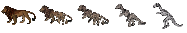
The measured durations for the tested pairs of models are given in the table 1. Three pairs of models were tested: the sphere and the Stanford bunny (both models have the same number of points), the African mask and the Christmas star, and finally the lion and the dinosaur. The measured times correspond to the fact that the asymptotic complexities of all tested clustering methods differ only in constant.
We have decreased the computational complexity and the total time spent by finding the assignments by allowing to store the once found assignments of points to file and then load it again.
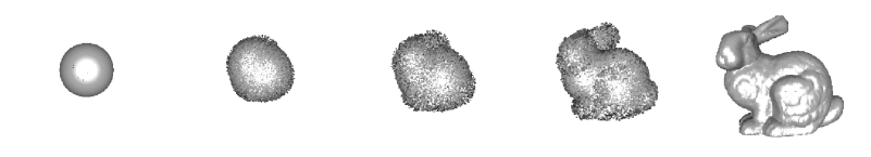
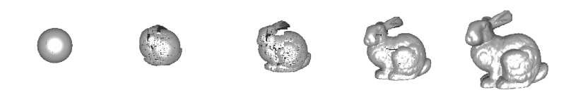
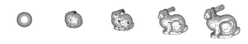
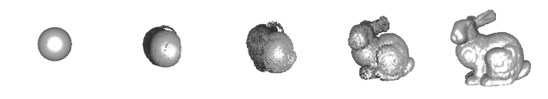
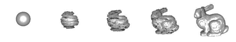
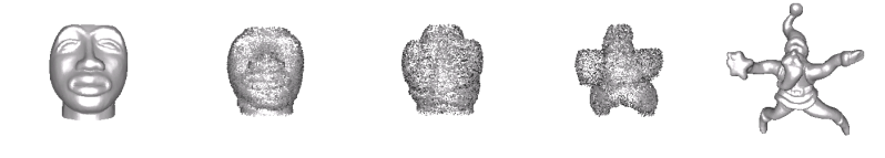
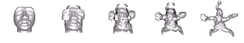
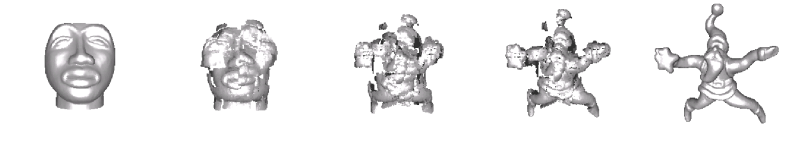
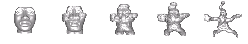
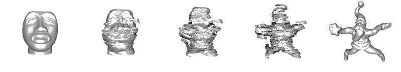
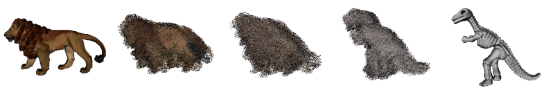
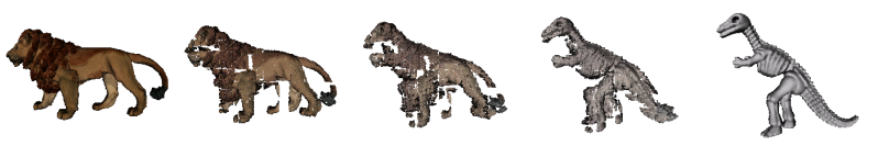
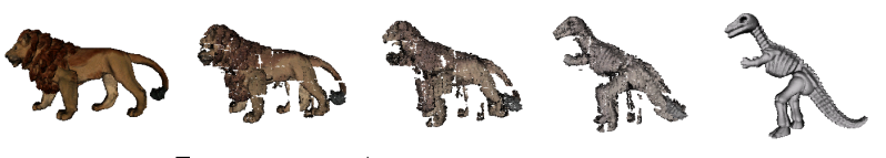
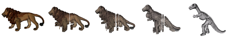
The progress of morphing of the tested pairs of models using various clustering methods is shown on the figures 6-10 (morphing of the sphere to the bunny), figures 11-15 (morphing of the African mask to the Christmas star) and the figures 16-20 (morphing of the lion to the dinosaur). Besides four tested clustering methods (orthogonal clustering, orthogonal clustering with random noise, bounding box division, covariance analysis) there is also shown for the sake of comparison the case when the assignment of points is chosen randomly.
|
In this section we will discuss the problems that provides the implemented methods. The main problem is the occasional occurrence of cracks in the model during the morphing. The cracks occur because of the space partitioning and the non-convexity of the shape. Our opinion is that this problem can not be eliminated only on the assumption of the sum of squared distances as the criterion of quality. This criterion is usable only for convex shapes. In a convex shape every surface point can be connected with every other surface points with a line without intersecting the surface of the shape. If a convex shape is divided by a split plane then the results are always two convex shapes. On the other hand a non-convex shape can be divided by a split plane to any number of convex or non-convex shapes and this is the main reason for the occurrence of cracks, see figure 5.
|
Alexa et al. have presented in [3] methods for transformation of a non-convex B-rep shape to a convex shape. The 3D manifold objects are homeomorphic with a sphere, so the unit sphere is the convex shape on which the non-convex shapes should be transformed. Those methods can be adapted for the point cloud representation.
One class of shapes are the star shapes. For a star shape exist at least one point O inside the shape which can be connected with every boundary point of the shape with a line without intersecting the surface of the shape. The point O is called origin. If the coordinate system is transformed to be the origin O in its center and the coordinates of each boundary point normalized then the star shape has been transformed to the unit sphere. The main problem is to find whether a shape is a star shape or not and find the origin O, especially for point cloud representation where no information about the surface is included.
Second class of shapes are non-convex non-star shapes. This class of shapes can be transformed to unit sphere using the barycentric mapping. The barycentric mapping uses a simple idea that every point is placed in centroid of its neighbors. The shape should be down-sampled until it is a convex shape. The coordinate system should be transformed to be the centroid of the shape in its center, then the coordinates of the points should be normalized, and the down-sampled points should be up-sampled on unit sphere respecting the idea of barycentric mapping.
In this case the paths can not be lines. The paths should depend on function which transforms the non-convex shape to unit sphere.
These problems are rather non-trivial ones and the future work will be focused on these particular problems.
For convex or just a little bit non-convex models gives the best results the morphing based on the orthogonal clustering. The generally best method for non-convex models can not be chosen. The testing has proved that the results of all methods depend on the shapes of the source model and the target model.
These methods are not usable for high-quality morphing, so the methods have to be improved. The sum of squared distances can not be used as only criterion of quality for non-convex shapes. Non-convex shapes have to be transformed to convex shapes.
[1] Pauly, M.; Gross, M.; Kobbelt L. P.: Efficient Simplification of Point-Sampled Surfaces, IEEE Visualization, 2002
[2] Alexa, M.; Behr, J.; Cohen-Or, D.; Levin, D.; Silva, C. T.: Computing and Rendering Point Set Surfaces, IEEE Transactions on Computer Graphic and Visualization, 2002
[3] Alexa, M.: Mesh Morphing STAR, Eurographics 2001 State of the Art Reports, Eurographics, 2001
[4] Pfister, H.; van Baar, J.: Surfels: Surface elements as rendering primitives, In Proceedings of SIGGRAPH 2000, pages 335-342, SIGGRAPH, 2000
[5] Zwicker, M.; Pfister, H.; van Baar, J.; Gross, M.: Surface Splatting, SIGGRAPH, 2001
[6] Rusinkiewicz, S.; Levoy, M.: QSplat: A Multiresolution Point Rendering System for Large Meshes, In Proceedings of SIGGRAPH 2000, SIGGRAPH, 2000
|
|
|
|
|
|
|
|
|
|
|
|
|
|
|