Abstract
Driving simulations are a good example of applications that utilize a dynamical model in a simulated environment. Such simulations can be decomposed into a graphical model responsible for rendering a specific space-configuration of entities within a virtual world and a dynamical model responsible for determining the evolution of this configuration over time. This paper wishes to address some important aspects of building these two models, with emphasis on their cooperation.
Keywords: virtual reality, vehicle dynamics, computer games, terrain modeling, numeric integration, dynamical modeling
1 Introduction
1.1 On Virtual Reality
The creation of convincingly realistic virtual worlds is without doubt one of the ultimate goals of computer graphics. The virtual world in question could be considered convincingly realistic if the resolution of its presentation were higher than that of the corresponding sense of human perception. Even though we are far from achieving this goal today, it is nonetheless a valuable and challenging experience to take part in maintaining the co-evolution of hardware and software towards the final goal of virtual reality.
There are two different aspects of creating virtual reality from the viewpoint of computer graphics. One of them is the realism of each rendered view of the world (often called a frame) as a stand-still image and the other is the realism of motion represented by a sequence of frames. While the field of computer graphics is concerned mainly with the former problem, a virtual world of interest would preferably be interactive and therefore require proper modeling of motions. As motions in the real world depend on the laws of Newtonian dynamics, it is straightforward to incorporate an element – a physical model – that represents an applicable partition of the laws of physics into the virtual world. Unfortunately dynamical simulation of numerous concurrent phenomena cannot be achieved on reasonable hardware, thus the main goal of many applications is to model only one (or few) aspect of the physical world in detail. Such applications, that contain a virtual world, are interactive and present a detailed dynamical model of an entity in question, are commonly called simulators in computer entertainment. This paper addresses some issues of creating such applications.
1.2 Simulating Driving
There is a growing home industry of writing driving simulations today [1]. This fact can be related to two factors. Home computers are becoming powerful enough to simulate vehicle dynamics in real-time without the need of writing bit-by-bit optimized code. Also vehicle dynamics is doubtlessly a field of wide interest among the laymen of driving, even more so with the professionals.
Apart from sheer entertainment a driving simulation is probably the best choice to represent the benefits of simulators in general: it is easily adaptable as a teaching and/or testing tool that driving students and racing teams can use with greatly reduced cost and caution compared to the real thing. Provided, of course, that the simulation is realistic enough to be of any professional use. This is why the professionals of vehicle dynamics also take interest in producing specialized models for real-time computing.
2 Aim and Scope of the Simulator
2.1 Entertainment
The driving simulation under design described in this paper is intended for entertainment purposes on a personal computer. This means that the quality of the physical model does not aim to meet engineering standards; nonetheless it wishes to be as realistic as it can be given a certain hardware configuration, through iterative refinement. The first goal is to design a coarse simulation engine with sufficient flexibility and modularity to be refined module-by-module without disturbing the underlying structure of the software.
2.2 Platform Issues
Although it is generally not advisable to design software for hardware not available at the time of the intended completion of the project, programs in the domain of computer graphics could be regarded as an exception. The evolution of computer graphics is so fast and we are so far away from the intended goal of virtual reality that any successful new attempt that aims at this goal renders all previous ones obviously out-of-date.
Therefore an amount of foresight is necessary to produce a piece of software with any chance of longevity. But since the general public surely does not have state-of-the art hardware, a well-designed program should exhibit massive scalability in order to provide an acceptable solution to a fairly wide range of users. Portability also poses a design issue; the reusability of code is a great advantage if we are to address customers using multiple computational platforms.
Fortunately there is a graphics library designed with many of the above-mentioned goals in mind: the OpenGL graphics library [2]. It is very advisable to use such a library in current attempts of creating a real-time graphics application. OpenGL is well designed, flexible, efficient and sufficiently platform-independent. Unfortunately it has at least one major drawback: any new features provided by vendors of graphical accelerator hardware are first only available in a vendor-specific fashion, which counters somewhat the intended platform independence.
The programming language of the author’s choice is C++, which is widely accepted as a tool for creating modular, portable code with good performance.
2.3 Decomposition of the Task
The task of writing a driving simulation can be decomposed into two partitions. One of them is to create the graphical model of the virtual world; the other is to create the physical model of vehicle dynamics. This paper is focused mainly on the latter task, but there are certain aspects of the former one that we wish to talk about. It is important to see that the two components have to work in concert to enhance the notion of reality in the virtual world. Quite often this is not the case in driving simulations, the graphical model represents only vaguely the happenings between the car and terrain and within the car. Upcoming simulations (such as the awaited Colin McRae Rally 3) put increasing emphasis on this idea, showing that the time is nearing when personal computers reach the power sufficient to cope with such issues.
3 Key Features of the Graphical Subsystem
3.1 Terrain Modeling
The idea of virtual reality introduces a world where the user can freely move in preferably all directions. Because we intend the driving simulation to aim towards this idea, it is not favorable to choose a world model corresponding to the average driving simulator, which contains only the track and its close surroundings.
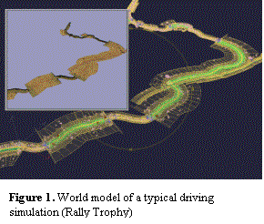
Instead of this we could base the virtual world of the
simulation on terrain modeling. The most common approach to do this is to
utilize a regular grid where we present height data at the points of the grid.
Such a height-field can be represented as a grayscale bitmap where the
whiteness of the pixels corresponds to height.
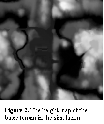
Such a height-map easily lends itself to be interpreted as a
quad patch. The main problem is that the amount of data present in the whole
map quickly becomes far too much to render without some form of culling and
Level Of Detail (LOD) scheme as the size of the map grows to represent larger
worlds. There are many sophisticated approaches to this problem such as SOAR
[3]. These methods require active participation of the CPU to deliver an
optimal set of triangles.
In an application such as a driving simulation we wish to devote the CPU to other tasks such as the evaluation of the physical model, so we are searching for a method we can use to coarsely partition the terrain data into larger blocks and then feed them to the GPU. Willem H. de Boer describes such a method [4]. His solution uses a quad tree structure to partition the terrain data by recursive quartering to some predefined depth. Multiple resolution versions are created from the smaller terrain blocks achieved by the subdivision. The quad tree containing the terrain data also contains the dimensions of each referenced terrain partition in its nodes.
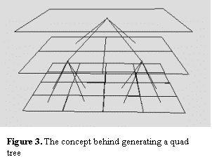
During rendering the tree is parsed, the bounding box for each
node is compared with the volume of the viewing frustum and the node is
rejected if there is no intersection between the two. At the leaf nodes
determined to be at least partly visible, one of the different LOD versions of
the block are chosen for display according to a complex distance metric that
incorporates the roughness of the terrain block. The different versions are all
ordered grid representations with different powers of two resolutions. The
possible effect of cracking when two blocks of different resolutions meet is
resolved by decreasing the resolution of the higher LOD block at its edge. This
problem is easily solvable if there is only one LOD change between the
neighboring blocks.
The current solution utilizes the ideas of de Boer, with the simplification that the more complex distance metric is replaced by simple distance. Each LOD version of each block is chosen for display if the distance from the center of the block to the camera falls between two predefined values.
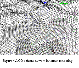
3.2 Spline-Based Smoothing
The described method of rendering the terrain data leaves open the question of how to determine the height of the terrain at an arbitrary point. Some sort of interpolation is clearly required between the heights of the neighboring grid points. This is the place where the interaction of the graphical and physical models comes into play: the vehicle dynamics model requires the height of the underlying terrain to be determined at the contact patch of each wheel. As real terrain changes height more smoothly than a triangulated surface, it is reasonable to use some higher order method of interpolation. Also, the surface normals are needed in the dynamics model as well as in lighting, once again in the arbitrary position of the wheel contact patches.
An approximation type B-Spline surface [5] using the grid points of the original terrain data as control points has the required properties, it is smooth, monotonous and its surface normals can be obtained analytically. Introducing the trick of only evaluating one coordinate (height) with respect to the other two (position on a plain), the calculations of a given point can be made efficient.
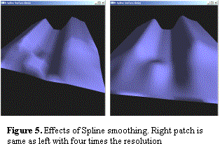
Once we have a smooth terrain representation it is
straightforward to use it as a basis for higher tessellation in rendering. We
can preprocess new LOD versions of each terrain block to a level allowed by the
available RAM, and we can produce more detailed tessellation on the fly, if
required.
If we wish to incorporate roughness on the centimeter level into the model, we can do so by introducing large-scale detail displacement maps added on top of the normal terrain data. These can be visualized using shader code for bump mapping or by tessellation in the case of extreme close-ups [6].
Apart from height and color, practically any property of the terrain surface with local relevance can be represented and interpolated using textures. The program currently takes benefit of a general Spline-evaluator class in calculating the macro and micro height variation of the terrain, the local friction coefficient and the color of the dust and kickup produced by the car.
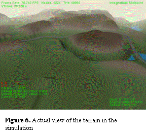
It is important to state that the resolution of the graphical representation of the terrain must be high enough to avoid such artifacts as submerging or floating wheels. It is also important to see that the ideas represented here address only a small portion of the issues encountered in designing a virtual world for a driving simulation. Most of these issues would easily require a separate paper each to discuss properly, such as the representation of dense vegetation, water, shadowing, atmospheric effects, clouds, dust, particles etc.
4 Key Features of the Dynamical Subsystem
4.1 Basic Methods
There are two basic approaches to simulating Newtonian dynamics, with different fields of application and validity. One of them is the numeric integration of equations that change rather smoothly over time and space [7] and the other is based on calculating impulse forces during sudden and rapid changes in motion of bodies [8]. The latter approach is mainly used to resolve collisions. Although it is a very important and valuable tool in handling such cases, in a driving simulation it is applicable only for handling the collisions of the car body with the ground and other obstacles, which is clearly not the foremost important task in deriving a model for vehicle dynamics. Therefore in this paper we wish to concentrate only on the integrative methods of evaluating a dynamical model.
It is important to note that the integrative method of doing a physical simulation gives only a framework, not a physical model in itself. The impulse based collision resolution does represent an actual physical model that needs only parameterization to work, but its applicability is more limited. The impulse-based method is generally used together with an integrative model to handle special cases. The smooth evaluation of the model is stopped once a collision situation is found and the state variables are updated instantly. Then the general simulation is restarted.
4.2 Object Representation
The bodies in the model are considered rigid, at least for the major part of the simulation. (Deformation due to damage caused by collision is not handled yet, but is intended to be in the future.) Rigid body dynamics is a well-established field of mechanics, with the advantage of relatively low cost of calculations (as compared to deformable bodies).
Rigid bodies are capable of two types of motion: linear and angular (rotational), which can be handled independently. In accordance with this, bodies have two sets of properties, their inertia and inertia tensors. Inertia or mass is the property that shows how the body responds to forces. Inertia tensors represent the spatial distribution of the mass of the body, and show how it responds to torques and characterize its rotation when “left alone”. Inertia is a scalar value that is constant unless the body gains or loses weight, such as if a body breaks up into smaller pieces. An inertia tensor, on the other hand, is a 3 x 3 matrix that changes with the orientation of the object in world space (hence the name tensor). The inertia matrix of an object in an arbitrary orientation can be computed using the following formula [9]:
![]()
where Ibody is the inertia tensor given in
the body coordinate system, and R(t) is the rotation matrix representing
the current orientation. There is a theorem stating that there exists an
orientation for every rigid body where its inertia tensor can be represented by
a diagonal matrix. It is advisable to use this orientation as the basis of the
body coordinate system, for it allows us to store Ibody as a
three-vector and its inverse as the element-by-element inverse of Ibody.
Apart from properties, each physical body in the simulation has 4 state variables:
r(t) – position,
P(t) – linear momentum,
R(t) – orientation,
L(t) – angular momentum;
And two auxiliary state variables:
v(t) – velocity,
ω(t) – angular velocity.
Each of these variables is a three-vector except for R(t), which is represented by either a rotation matrix or a quaternion. The auxiliary variables are computed via the following equations:

written in a fashion to emphasize the analogy. While v(t) is constant in the case of an undisturbed object (that no external force is exerted upon), that is not true of ω(t). The respective moments are both constant under such circumstances. The management of R(t) and I(t) is the only real challenge in the framework, apart from them the rest of the dynamics is pretty straightforward. This approach is referred to as six degrees of freedom modeling (6DOF for short) because of the three axes and three angles of possible motion.
4.3 The Simulation Cycle
Given the above framework the real problem in creating an adequate simulation is the physical model itself: a set of differential equations (ordinary differential equations, or ODE-s to be precise) enabling us to evaluate the forces and torques governing the motion of objects in the given time and space. The equations may depend on any obtainable property of the object or the virtual world, but are preferred to behave smoothly, i.e. without rapid changes for small variations in the input space. Suddenly appearing huge forces are almost certain to cause problems with most types and stepsizes of numeric integration.
Rephrasing the main idea of the previous paragraph, we require the physical model to provide us for each object with a (limited) number of forces (Fi) and the points of their application to the object (ri). The effective forces and torques result from these two simple equations:

In practice, the physical model is generally partitioned into many smaller modules with their effects summed using force and torque accumulators that are zeroed at the beginning of each evaluation step.
So far we have a state representation of the virtual world and proper functions to evaluate the forces acting on it in a given instant and configuration. (These functions – or the following – seldom take the form of a differential equation in working code, only on paper at design time.) Now we wish to obtain the state of the system at some later time. We have the basic equations of Newtonian dynamics to guide us:

and also

the last equation being valid for the quaternion
representation of orientation as derived in [9].
It follows that to obtain valid state variables for time t we have to evaluate the expressions:
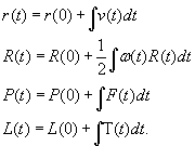
Unfortunately analytic integration is only possible in very simple or special cases. The general approach is to use numeric integration: iteratively updating the state variables at discrete time steps. Numeric integration works by sampling the forces in effect at least once during each time step, and using this finite-resolution information to calculate the resulting changes. It is to be seen that this scheme – no matter how sophisticated an integration method one uses – generally results in numeric errors of a magnitude characteristic of the method, causing numeric drift. There are certain cases where we are bound to encounter this problem, as mentioned above.
The most basic mode of numeric integration is Euler’s method, which regards the force, torque, velocity and angular velocity to be constant during the time step. This corresponds to a first-order Taylor-series representation of the system, thus it is called a first-order method. State variables are updated using the following equation:
![]()
This method is very simple, fast and easy to use. Unfortunately it has an error of Ο(Δt2) and does not even give correct results in its simplest form for constant forces. The greatest problem with it is probably that it drifts very rapidly in the case of strong undamped spring forces and easily causes undesired explosive effects in the physical model. Therefore it is favorable to introduce higher order numeric integration to the physical framework, at least as an option.
There are two widely used higher order methods of numeric integration, one of them is the second-order midpoint method, the other is the so-called fourth order Runge-Kutta method (RK4) [7]. These have errors of the order Ο(Δt3) and Ο(Δt5), and require the underlying physical model to be evaluated 2 and 4 times respectively. While RK4 is the virtual industry standard for doing dynamical modeling, in the case of a computer game the required precision is not as high as in engineering applications. The main issue is preventing explosive physics, and the midpoint method does an excellent job of that: it is analytically correct for a range of forces and greatly enhances the stability of modeled spring forces.
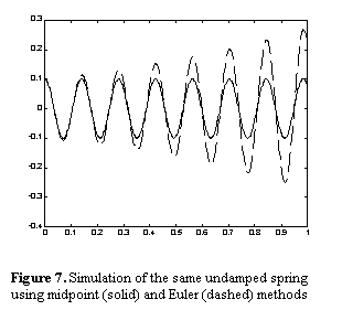
The midpoint method - as derived in [7] - works by calculating the Euler step, then using the evaluation of the model again at the midpoint of the Euler step to update the state variables. In a more mathematical fashion, this procedure can be written as:
![]()
The current version of the program supports all three types of
integration with emphasis on the midpoint method. Although the physical model
does run noticeably smoother using methods of higher order integration, the
difference is almost negligible. This fact proves that some unrealistic effects
produced by the simulator are due solely to the vehicle dynamics model, not the
instability of numeric integration.
4.4 Constraints
So far we have said nothing about the derivation of the underlying physical model used to determine the forces at work in the simulation. Though not much can be said in general, there are certain approaches, which add a higher level to the methods described above. Constraint-based modeling is an evolving field concerned with forces resulting from geometric constraints in the model [10]. Such an approach is very useful in the case of vehicle dynamics for deriving forces in the suspension system of the car. The actual simulation does not make use of this method so far, but we wish to incorporate it in the future.
5 The Model of the Car
5.1 General Properties
The main duty remains of providing the actual model representing the car in the simulation. As stated before, the vehicle model in a game is not required to be as sophisticated as the one in an engineering application. Therefore we wish to outline a basic model, which is sufficient for running an entertaining simulation, but can be enhanced if desired.
The car is represented in the simulation by 5 rigid bodies, the car chassis and the four wheels. Besides these, logical objects exist in the simulation that only provide forces and torques while having no mass or shape of their own.
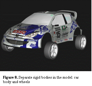
The car model has 6 DOF for the chassis, 3 for each front and
2 for each rear wheel, and one DOF for the rotation of the engine, giving a
total of 17 DOF. The wheel movement is limited to vertical motion in the body
frame of the car, rotation about its spindle axis and steering rotation in the
case of the front wheels (or all of the wheels in case of four-wheel steering).
The logical components of the model include the engine, clutch, gearbox,
differentials and suspension. The brakes are also a logical component, but they
are handled within the wheel model, by adding in a single torque value for each
wheel.
The car body itself has no real model currently except for providing penalty forces in the case of collisions between its bounding box and the terrain, which, although acceptable in results, is clearly not the state-of-the-art solution for collision resolution. Also air drag is accounted for in the model of the car body in a very simplistic manner. Air drag varies with the square of the velocity and does not depend on the orientation of the car (which is not true in real physics). Forces due to air drag (and gravity) are modeled to act at the center of gravity (COG) of the car, thus exert no torque on the body chassis.
The most important – and thus most complex – component in the dynamical model is the tire model, for it is clear that it ultimately determines the handling of the car and thus the realism of the simulation. The suspension model could be considered to be the second most important for similar reasons. Suspension parts actually move with respect to the car frame and thus have characteristic physical properties in a real car, but for our current purposes it is reasonable to regard them as logical components and lump some of their real physical properties to the wheels (also the inertial properties of the drivetrain) [8]. In the following sections we wish to give an outline of the logical components topped by the tire model discussed in a bit more detail.
5.2 Engine
The main property of the engine is a function of its maximum output torque at a certain angular velocity, often called a “torque curve”. It is represented by multiple linear segments and is normalized to be able to use engines of different power with the same characteristics. The effective multiplier is given as a separate value in the car’s configuration file.
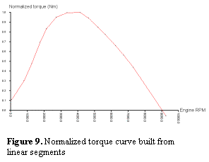
The engine uses the throttle position as an input variable.
The available torque is determined linearly from the throttle position, which
is a crude but sufficient estimation. The engine has rotational inertia (which
is a single scalar in this case) and frictional constants; its friction during
rotation varies roughly linearly with the angular velocity. The output torque
is fed to the clutch, which feeds back a response torque from the rest of the
drivetrain. Engine rotation is updated using the difference of these two
torques.
5.3 Clutch
The clutch has the purpose of negotiating differences in angular velocity between the engine and the rest of the drivetrain. This is important because we start up with a running engine and standing wheels, and need to smoothly eliminate the difference or else the engine would stall.
There are basically two types of clutch in the real world and the model: dry and viscous. Dry clutches work based on Coulomb friction, the clutch torque is roughly linear with the force applied between the clutch plates in case the plates are sliding on each other. When the rotation of the plates becomes equal (and the clutch is disengaged) the rotation of the engine and the drivetrain become linked. This link holds until the clutch is engaged or the torque between the plates exceeds a predefined level. Clutch control is automatic in the simulation; it automatically disengages if the engine revolution falls below a certain level.
As of viscous clutches, a proper model for coding them is yet to be found. The current solution derives torques using the difference between the angular velocity on the two sides of the clutch.
5.4 Gearbox
A gearbox has the task of converting angular velocities and torques in the drivetrain. It has a set of gears characterized by their ratio of conversion. These ratios are used for multiplying the torque and dividing the angular velocity from the engine to the wheels and vice versa from the wheels to the engine, based on the theorem that the product of the two must remain constant during the conversion.
There are two methods for changing gears: manual and automatic. Automatic gear change is based upon efficiency: the gear is switched to the neighboring higher or lower one if the absolute torque is higher in that gear compared to the current one. The efficiency of the torque output is decreased during automatic gear usage (as it is in real life) to give manual gears a benefit. The gearbox has control of the clutch during these operations.
5.5 Differential
The basic idea of a differential is much easier to implement in code than it is to build in real life. A differential has the duty of ensuring that all the wheels receive the same amount of torque while enabling them to rotate at different speeds. This is necessary because during a turn the wheels of the car cover different distances within the same time. In programming this can be accomplished by simply dividing the available torque at a preset ratio among the driven wheels. The angular velocity of the wheels is averaged to find the effective rotation of the drivetrain.
While the basic differential is “open” in the sense that it does permit limitless difference between the angular velocities of the wheels it affects, this scheme is not always useful. In the case of powerful racecars and off-road vehicles it is desired to limit the “slip” of the differential. The solution to this problem up to date is similar to that of the viscous clutch, which should be enhanced in the future.
5.6 Suspension
We have provided a rather simple solution to the suspension system of the car. Wheel suspensions are treated completely independently; also there is no camber variation with the suspension travel.
As only vertical motion is permitted for the wheel in the body frame of the car, the horizontal forces acting on the wheel are simply forwarded to the chassis itself. This gives acceptable results but completely neglects the real geometry of the suspension that is normally taken into account by the introduction of roll centers [11]. With the current solution roll centers of both the front and rear axles are set permanently at ground level, which increases the tendency of the car to flip over in some situations. This can be countered by using the vertical suspension force as the normal force in the tire model calculations; in this case two wrongs do make a right.
The vertical travel of the wheel is governed by two nonlinear sets of spring and damping forces, one of them reserved for the bump stop (a piece of strong rubber that stops the suspension movement at the point of maximum suspension travel). Spring forces depend on the vertical position of the wheel in the car frame and damping on its velocity. These forces are applied to both the car chassis and the respective wheel.
5.7 Tire Model
As mentioned above, the tire model of a driving simulation is the single most important feature of the dynamical model. This should be evident because under normal circumstances only the tires of the car touch the ground and therefore all major forces acting upon the car body ultimately originate from the tire. The tire model is responsible for traction and cornering forces and thus determines the handling characteristics of the car, and how the engine torque is translated to acceleration. The tire model is simplified to the generation of three components: normal, longitudinal and lateral forces. The latter two forces are decoupled to the maximum extent possible and then combined to meet the limits set by a friction ellipse. Aligning moment is currently neglected because no means of force-feedback have been introduced to the simulation.
Modeling tires in real time is widely agreed upon by professionals to be a difficult problem. Tire models are either purely analytical or semi-empirical, representing functions to fit experimental data. Both types of models can be steady-state or dynamical, with a different range of validity concerning the domain of frequencies encountered by the tire. For the macro height variation of the terrain a steady-state approach is sufficient, and the simulation currently utilizes such a model. With the recent introduction of the displacement height-maps the validity of such a solution decreases but fortunately any steady-state model can be extended to a dynamical one with the introduction of two new state variables [11]. This is to be done in the near future.
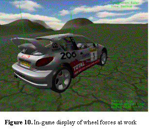
Steady-state tire models generally calculate traction and
cornering forces based upon two properties of a wheel in motion: slip ratio and
slip angle [11][12]. To understand these properties it must be made clear that
the tire generates forces due to its deformation best represented by complex
nonlinear spring forces. A tire producing traction (or braking) forces has
different angular velocity as compared to the same tire rolling freely at the
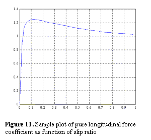
same traveling speed. This difference is characterized best by slip ratio, which
is defined by:
![]()
where ω is the actual angular velocity of the tire and w0 (=vx/Reff,
Reff is the effective radius of the wheel) is the angular velocity of a
free-rolling tire moving with the same linear velocity as the driven or braked
tire. Slip angle (SA) is the angle between the wheel plane and its direction of
motion.
The industry standard for tire modeling in real-time applications is the so-called Magic Tire Model of Pacejka [11][12]. It is a semi-empirical model recognized to be exceptionally correct for derivation of tire forces under explicit circumstances. Unfortunately its parameter set is rather complex and cannot be modified intuitively to account for changes in the tire or the type of surface the tire rolls upon (since it would require different, hard-to-obtain experimental data sets for each case). Even though we wish to implement the Magic Tire Model in the future (because of its applicability on tarmac), we were concerned with finding an analytical model due to these issues. Finally we chose to implement a tire model based upon that of James Lacombe [9].
Lacombe’s model is an analytical steady-state model. It focuses on clearly distinguishing two regions of the tire contact patch, a static (sticking) and sliding region. The sliding region is handled based upon a Coulomb-type friction model and the static region based upon linear and nonlinear spring forces concerning the longitudinal and lateral forces respectively (the normal force is also generated from a nonlinear spring very much similarly to most of the models). The strength of the model lies in its approach to the derivation of forces during combined longitudinal and lateral acceleration, while the discreet cases produce results similar to those of other tire models. The ratio of the static and sliding regions varies smoothly during the simulation and the sliding region produces longitudinal and lateral forces in a coupled manner since a Coulomb-type frictional force always acts against the direction of sliding motion, in this case the motion of the contact patch on the ground. (The direction of motion of the contact patch is normally not the same as that of the wheel, only if the wheel is completely blocked and does not roll at all.)
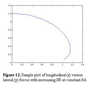
While the model at work in the simulation is not the most
sophisticated one possible and wishes to be enhanced in the future, it does
respond lively to parameter changes and driving style. Important real-world
effects such as turn-in braking and power oversteer can be produced with ease
in the simulation, along with other cases of under- and oversteer. Handling
differences between front-, rear- and four-wheel driven vehicles are very
pronounced and probably even exaggerated to some extent. On the whole the car
behavior is quite realistic compared to the simplicity of the model.
It is important to note that determining the validity range of the parameters in the model is in cases almost as hard as deriving the model itself and accounts for a major part in the realism of the final product.
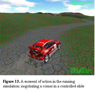
A video sequence from the running game (divx)
6 Summary and Future Work
It is rather challenging to write a driving simulation. In this paper we have made an attempt to outline some basic ideas in the design of such an application. We have sub-classed the original task into two fields: graphical and physical modeling. We have introduced an adequate terrain representation; a general framework for doing physically based modeling and the actual physical model of the car. These three aspects serve as a basis for building a more sophisticated simulation.
The list of things that can be done to enhance the application is virtually endless, limited only by time, imagination and computing power. The terrain model greatly desires objects and vegetation to add to its visual realism, while these objects should also be modeled physically to enhance the connection between the graphical and physical representations. The impulse- and constraint-based methods should be introduced to the physical model. Car body deformation due to collision should be addressed. The tire model should be enhanced and extended to a dynamic one. Real suspension geometry should be modeled. And last, but not least driver AI should be introduced to enhance the playability. The simulation - according to our intentions - is far from complete as is well shown by its current version number: 0.1.0.
References
[1] R. van Gaal. Racer Project. A brief list of home-made driving simulations on the internet www.racer.nl/links.htm
[2] M. Segal and K. Akeley. The OpenGL Graphics System: A Specification (Version 1.2). Silicon Graphics, 1998
[3] P. Lindstrom and V Pascucci. Visualization of Large Terrains Made Easy. IEEE Visualization, 2001. Obtained from www.vterrain.org
[4] W. H. de Boer. Fast Terrain Rendering Using Geometrical Mipmapping .flipcode, 2000. Obtained from www.vterrain.org
[5] L. Szirmay-Kalos. Computer Graphics. ComputerBooks, Budapest, 1999 pages 48-59
[6] NVidia OpenGL SDK. NVidia Corporation, 2001 www.nvidia.com/developer
[7] A. Witkin and D. Baraff. An Introduction to Physically Based Modeling: Differential Equation Basics. Robotics Institute, Carnegie Mellon University, 1997
[8] D. Baraff. An Introduction to Physically Based Modeling: Rigid Body Simulation II – Nonpenetration Constraints. Robotics Institute, Carnegie Mellon University, 1997
[9] D. Baraff. An Introduction to Physically Based Modeling: Rigid Body Simulation I – Unconstrained Rigid Body Dynamics. Robotics Institute, Carnegie Mellon University, 1997
[10]A. Witkin. An Introduction to Physically Based Modeling: Constrained Dynamics. Robotics Institute, Carnegie Mellon University, 1997
[11]E. M. Lowndes. Development of an Intermediate DOF Vehicle Dynamics Model for Optimal Design Studies. Ph.D. Thesis, Department of Mechanical and Aerospace Engineering, Raleigh, 1998
[12]J. Lacombe. Tire Model for Simulations of Vehicle Motion on High and Low Friction Surfaces. Proceedings of the 2000 Winter Simulation Conference, pages 1025-1034