Image Processing for fine arts
Abstract:
The contribution deals with image transformations applicable to the fine arts and to the correction of photographic images. The program includes image filters for image blurring, correction of the shade value, softening of the drawing - blurring, rotation and various special and deformation effects, e.g. map relief of the image, effect of an oil painting, solarization, fish eye effect or whirlpool and other interesting transformations. The library of these special image filters is focussed on the application to user's programs.
By means of this library, interesting and useful transformations of actual images can be produced which may extend the limits of the mere entertainment.
Contents
2. Mathematical principle of raster image transformation
General description of raster transformation
3. Description of implementation
One can hardly find any answer to the question "What is computer based fine arts?". Creative arts that use the computer as its media is used in various other branches of art, such as music. In any case, computer is used as a tool for creation - instead of brush one uses mouse. Herbert W. Franke, one of the inventors of computer art, touched this subject in this question: "Is the image created using computer really an art?" We could also ask whether tones played using violin are also music. In both cases we just used tools to produce the art.
In some tasks, computer is more suitable than traditional artistic tools. An example of such task is filtering and geometrical transformation of an image. It could be expected, that some time the expression "Computer Art" will be dead, but the technology is not the key point to the art - the human is - when equipped with some technical means.
Clearly, oil painting is always done on the paper or cloth using brush and colors. The purpose is not that the filter when applied to a photograph creates painting, but that the filtered image has nice and interesting appearance.
The above situation resembles the situation with traditional and digital photography. The fact that digital photographs could be easily grabbed, archived, marked, transferred through telephone lines, etc. does not have to say anything to a creative user. The situation starts to be more interesting from the moment when it is possible to change the technical quality or layout of the image. Very few computer "amateurs" who have once "simply created" the effect of plastic relief know how difficult it would be to do similar effects using traditional photography. It would be necessary to produce both positive and negative versions of the image, then offset them a little, and finally expose on the positive photographic paper. After the paper is developed, the image (hopefully) shows the plastical effect. The fancy "solarisation", that is traditionally produced with difficult to control overexposure, can be easily simulated on a computer. Now, it is not necessary to use special lenses to produce "soft" images. Moreover, filters can be applied to the image at any time.
The differences in the processing are straightforward. Using the digital technology, every change to the image can be seen on the screen more or less immediately. If the user does not like the changes, he can revert them usually by pressing single button. The costs of material are zero evens when the most complicated operations are performed. Changes of colors, brightness, or contrast cost only a little bit of electricity. Moreover, most of the image processing programs offers functions that are not possible to do with a standard photography at all, or that have very high technological requirements.
Several image-processing programs are available on the market in these days, like Adobe Photoshop, Aldus Gallery Effects, PhotoFusion, or Aldus Photostyler. However, none of these programs offers its functions to be used by other programs. Unfortunately, literature describing special image transformations is also nearly non-existent.
This contribution describes a library that offers programmers a possibility to use several image-processing algorithms, like sharpening, softening, several brightness corrections, and special geometrical and other transformations.
The purpose of all the filters is to make the work of professional photographers Easier and allow them to correct the digital photographs in a simple way. They can improve damaged images, sharpen the images that require improvement of resolution, or do the opposite to achieve artistic impression. It is also possible to lighten or darken the image, create a negative image, or clip the image with arbitrary shape.
The library contains filters that have purely artistic effect. These can convert photographed images to images that look like that they have been painted, increase a granularity, deform them, or change their appearance in a way that they look like seen in a broken mirror. Effect of a lens or fish eye are achieved by projecting the image on a spherical surface, also available are geometrical transformations as skew, zoom, etc.
All the effects mentioned above are contained in a single library, which is implemented in C++ and which is platform independent.
2.
Mathematical principle of raster image transformationGeneral description of raster transformation
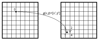
The transformation of a raster image is based on the transformation function, which assigns the values calculated from the original raster values to the new raster. It means that each point [x,y]of the new raster is assigned a value of the transformation function corresponding with the original raster.
|
|
New[x,y] = f(Old[i,j]) iÎ á 0..X) , jÎ á 0..Y) , |
(1) |
Where f is the transformation function, X and Y are the width and height of the original raster, resp. and [x,y] are the Cartesian raster coordinates. New is the identification of the new raster and Old is the identification of the original raster. The equation (1) is valid for each point [x,y] of the new raster where
x
Î á 0..NX), yÎ á 0..NY),NX is the width and NY is the height of the new image (they may, but not necessarily, be identical with the X,Y values of the original image).
For the transformation
|
|
g(x,y) = [x',y'], |
(2) |
Where [x,y] are the coordinates of the original raster and [x',y'] are the coordinates of the new raster a situation may occur where x',y' are values of a real type which means that the value of the [x,y] point of the original image Old[x,y] must be distributed over the neighboring points of the raster by means of an interpolation function.
[nx,ny], [nx+1,ny],
[nx,ny+1], [nx+1,ny+1],
where it is valid that
|
|
nx < x' < nx+1, ny < y' < ny+1 . |
(3) |
Fig. 1.
|
|
Old |
New |
|
0 = [x,y], |
0'= [x',y'], 1 = [nx, ny ], 2 = [nx+1,ny], 3 = [nx,ny+1], 4 = [nx+1,nx+1]. |
The resulting value of the [x',y'] point must be interpolated into the points 1,2,3,4 of the new raster .
Mathematical notation of raster filters
Many of the raster transformations may be described by mathematical equations. The conventions for the description of these operations will be given.
X,Y
- dimension of the rasterA
- maximum angle of the polar coordinates (here 360°),R
- maximum radius of the polar coordinatesZ
- maximum point intensity%
- operator modulo,[x,y]
- Cartesian coordinates of the raster point{r,a}
- polar coordinates of the raster point , r is the radius (distance from the center) and a is the angle.Old[x,y]
- value of the color of the original image in the [x,y] pointq(x,y,N)
- value of the most frequently used color in the original raster from the [x-N,y-N] to the[x+N,y+N] pointThe transformations will be recorded in the following form:
|
|
New[x,y] = f(Old[dx,dy]) , |
(4) |
kde y = 0..Y, x = 0 .. X.
In the transformations the Cartesian coordinates are converted to polar coordinates and vice versa:
a = atan(y/x),
r = sqrt(x2 + y2),
xval = r * cos(a),
yval = -r * sin(a).
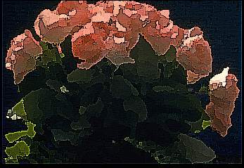
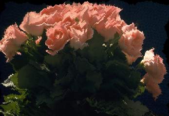
Effect of an image painted by oil (Oil)
The following equation refers to this effect:
|
|
New[x,y] = q(x,y,N) , |
(5) |
Where N
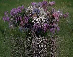
equals 1..5.Effect of a random shear image (Shear)
This effect is difficult to be described by an equation:
|
|
New[x,y] = Old[dx,dy] , |
(6) |
Where the dx,dy differ from the previous dx,dy values (in the previous point) by o ± 1 (at random). An impression of an image waved at random in both directions is created.
Effect of the random shifted image parts (Slice)
This the equation for this effect:
|
|
New[x,y] = Old[x+xshift[y],y+yshift[x]] , |
(7) |
Where the xshift,yshift values represent the random shifts in the range of ± 31 in blocks from 8 to 39 points at random in both directions.
Melt Effect (Melt)
An impression is made of an icy image, which is melting. This transformation first requires the copy of the original image (it operates in situ):
New[x,y] = Old[x,y]
,The x, y coordinates are chosen at random for which the following is true:
:
|
|
If New[x,y] Ł New[x,y+1], then swap(New[x,y],New[x,y+1]), |
(8) |
Where swap is the function for values exchange. This is repeated for the total number of the raster points.
Tile Effect (Tile)
The image is divided into square parts of a constant size which are distributed at random distances from the original site:
|
|
New[dx+ox,dy+oy] = Old[dx,dy] , |
(9) |
Where dx passes from x to TileSize and dy passes from y to TileSize, where x,y are the multiples of TileSize. The ox,oy are random values in the range of ± 16 and they are constant for a particular section of the raster.
Matte Effect (Effect of the inversive image thresholding)
The image according to the GAMMA value is inversibly thresholded:
|
|
New[x,y] = lookup[Old[x,y]] , |
(10) |
Where the following is defined for each color:
lookup[color] = (Z*(color/Z)GAMMA < 3.0)? Z : 0
.Gamma Correction (Intensity Correction)
Mathematical equation for this transformation:
|
|
New[x,y] = Old[x,y]*Koef , |
(11) |
If koef>1
, the image intensity increases, if Koef<1, the image intensity decreases.Negative Image (Negative)
One of simple transformations:
|
|
New[x,y] = Z - Old[x,y] . |
(12) |
Cut Circle
The transformation is based on the circle equation:
|
|
If (x-X/2)2/(X/2)2 +(y-Y/2)2/(Y/2)2 < 1 Then new[x,y] = Old[x,y], Or New[x,y] = 0. |
(13) |
Image Solarization
Solarization process which disappears from the left to the right:
|
|
New[x,y] = (Old[x,y] > (Z*x)/(2*X)) ? Old[x,y]:Z-Old[x,y] . |
(14) |
Relief Map Effect
The plastic relief is created by the combination of the original and shifted half negatives:
|
|
New[x,y] = Old[x,y] + (Z/2 - Old[x+2,y+2]) . |
(15) |
Image Shrink
The coordinates of the original raster are multiplied by the coefficient:
|
|
New[x,y] = Old[x*Koef,y*Koef] , |
(16) |
where Koef > 1.
Effect of an interesting caricature (Caricature)
In this transformation, polar coordinates are used:
|
|
New[x,y] = Old{sqrt(r*R),a} , |
(17) |
Where sqrt is the root of the number.
Fish Eye Effect (Fish Eye)
The transformation results in a convex image.
|
|
New[x,y] = Old{r2/R,a} . |
(18) |
Swirled image Effect (Swirled)
Swirled image is formed by:
|
|
New[x,y] = Old{r,a + r/Koef} . |
(19) |
Cylinder Mirror Effect (Cylinder)
The upper edge of the raster is drawn to the center, the left and right edges are fused.:
|
|
New[x,y] = Old[a*X/A,r*Y/R] . |
(20) |
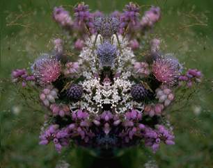
Horizontal Mirror Effect (Horizontal Mirror)
Depending on the value identifying the side, the left or right side may be reflected.
|
|
New[x,y] = x<X/2 ? Old[x,y]:Old[X-x,y] ,New[x,y] = x>X/2 ? Old[x,y]:Old[X-x,y] . |
(21) (22) |
Bathroom (Bathroom 2) Window Effect
These transformations are in [Holzm] called bathroom window views.
|
|
New[x,y] = Old[x + (x%32)-16,y] ,New[x,y] = Old[x + ((a+r/10)%32)-16,y] . |
(23) (24) |
Image Blur (Blurred Image)
The mean value of the surrounding points is calculated by this transformation.
|
|
New[x,y] = avr(x,y,N) , |
(25) |
Where avr(x,y,N)calculates the mean in the surrounding of the point [x,y] in the distance ± N/2.
Pixelized Image (Pixelize)
This transformation calculates the mean value of the surrounding points and poses this mean value to all these points:
|
|
New[x,y] = avr(dx,dy,N) , |
(26) |
where avr(dx,dy,N)calculates the mean in the [dx,dy] field , where the size of this field (area) is N2.
Filters defined using convolution masks
Basic equations for the operations with convolution masks:
The filters are defined by a matrix having dimensions either 3x3 or 5x5. This will be illustrated by the matrix which produces identity from the original image.
|
Mask: |
M = |
0 |
0 |
0 |
(27) |
|
|
0 |
1 |
0 |
||||
|
0 |
0 |
0 |
Calculation of the point value New[x,y]:
|
|
New[x,y] = |
Old[x-1,y-1] Old[x,y-1] Old[x+1,y-1] Old[x-1,y ] Old[x ,y ] Old[x+1,y ] Old[x-1,y+1] Old[x ,Y+1] Old[x+1,y+1] |
* M[1,1] + * M[2,1] + * M[3,1] + * M[1,2] + * M[2,2] + * M[3,2] + * M[1,3] + * M[2,3] + * M[3,3] |
(28) |
Some masks are assigned a coefficient koef, by which the resulting value should be divided, and some masks are, moreover, assigned the Bias, which is added to the resulting value:
|
|
New[x,y] = New[x,y]/koef + Bias |
(29) |
The koef and Bias values equal 1 and 0, resp. in other filters.
Edge detection
|
|
This filter is defined by three matrixes:
|
1 |
-2 |
1 |
(30) |
|
|
-2 |
4 |
-2 |
||||
|
1 |
-2 |
1 |
|
|
-1 |
-1 |
-1 |
(31) |
||
|
-1 |
8 |
-1 |
||||
|
-1 |
-1 |
-1 |
|
|
0 |
1 |
0 |
(32) |
||
|
1 |
-4 |
1 |
||||
|
0 |
1 |
0 |
Emboss filter
|
Bias = Z/2 value is set for this filter |
-1 |
0 |
0 |
(33) |
||
|
0 |
0 |
0 |
||||
|
0 |
0 |
1 |
Enhanced detail
|
The coefficient koef for this mask equals 6. |
0 |
-1 |
0 |
(34) |
||
|
-1 |
10 |
-1 |
||||
|
0 |
-1 |
0 |
|
Enhanced edges |
-1 |
-1 |
-1 |
(35) |
|
|
-1 |
9 |
-1 |
|||
|
-1 |
-1 |
-1 |
|
Enhanced focus |
-1 |
0 |
-1 |
(36) |
||
|
Koef = 3 |
0 |
7 |
0 |
|||
|
-1 |
0 |
-1 |
||||
|
Reduce jaggies |
0 |
0 |
-1 |
0 |
0 |
(37) |
|
|
0 |
0 |
3 |
0 |
0 |
|||
|
-1 |
3 |
7 |
3 |
-1 |
|||
|
0 |
0 |
3 |
0 |
0 |
|||
|
0 |
0 |
-1 |
0 |
0 |
Soften filter
koef = 99 |
11 |
11 |
11 |
(38) |
||
|
11 |
11 |
11 |
||||
|
11 |
11 |
11 |
koef = 100 |
10 |
10 |
10 |
(39) |
||
|
10 |
20 |
10 |
||||
|
10 |
10 |
10 |
koef = 97 |
6 |
12 |
6 |
(40) |
||
|
12 |
25 |
12 |
||||
|
6 |
12 |
6 |
|
Blur light |
1 |
2 |
1 |
(41) |
||
|
koef = 14 |
2 |
2 |
2 |
|||
|
1 |
2 |
1 |
||||
Implementation of image filters
So far, all the image transformations take into account the same size of the original and transformed snaps. Therefore the same variables for raster sizes are used for implementation:
Xsize
- raster widthYsize
- raster heightTherefore, the basic algorithm implementation is used for each transformation:
for y varying from 0 to Ysize
for x varying from 0 to Xsize
execute transformation.
Effect of an image painted by oil
The field of 256 items for histogram storage (number of the colors used in the section given) was necessary for this effect. In the environment (surroundings) of each point [x,y] in the range limited by the points [x-N,y-N], [x+N,y+N], the multiplicity of the colors used is stored in the field declared. After this, the most frequently used color is chosen out of this histogram and recorded into the allocated structure for storing the image to the [x,y] position. The algorithm is repeated for each item of the image raster in this way. To calculate the RGB components for the intensity in the range of 256 levels the following equation is used:
I = 0.299*r + 0.587*g + 0.114*b
.Effect of a random shear image
In the main cycle, the shift in the direction given, which is prepared in the allocated shift field yshift[], is added to each coordinate. This field contains random figures having maximum difference of ±1. The X-shift is calculated as early as in the main cycle.
Effect of the random shifted image parts (Slice)
For two declared fields, the shift of blocks in the range from 8 to 39 pixels is designed in two independent cycles. These blocks can be shifted by ± 31 points. In the main cycle only the precalculated shifts are added to the original coordinates. Three RGB image components are always presented.
Melt Effect
This effect operates "in situ" - therefore, an original raster copy must be first made in the allocated space. The program identifies the number of raster points (the number of transformation cycles). In each cycle the random x,y coordinates are chosen. The color value in this location is compared with that of the point chosen on the x,y+1 coordinates. If the value of the color under an accidentally chosen point is higher or equals the value of the point chosen, these two color values are interchanged.
Tile Effect
Both the immersed cycles increase the x,y values by the size of the TileSize section. In the interior of these cycles the random relative shift of these sections is calculated. After this, these shifts are added to the coordinates of the original image, and the complete parts are simultaneously transformed into the allocated memory. It must be also checked if the calculated shift does not happen to exceed the raster.
Matte Effect (Effect of the inversive image thresholding)
For the intensity level values, each level will be calculated from the equation given in the previous chapter (under the equation designed by (10)) or this intensity will be marked by white or black colors. These values will be stored in the field lookup[], to which each intensity of the original raster will be referred. The intensity which will be inserted as index into the lookup field is calculated from the RGB components on the x,y coordinates. The value in the lookup[] field will be assigned to the new raster in the x,y position.
Gamma Correction (Intensity Correction)
In the new transformation cycle, the original component multiplied by the coefficient given will be assigned to each RGB component. However, the exceeding of the value of the color component must be observed (if this occurs, maximum value of the component must be set).
Negative Image (Negative)
The new RGB components are assigned the value of the difference of the maximum component value and the original RGB component.
Cut Circle
The condition in the immersed cycle determines if the point is copied into the new raster or clear to zero depending on the fact if the point coordinates are situated inside the circle which is determined by the quotation with the parameters of the image size.
Image Solarization
The value of the image intensity is calculated for each point. This is compared by the equation (14). This condition being met, the original value of the RGB component is recorded. Otherwise, the inversion value of the component is recorded.
Relief Map Effect
Intensities are calculated for the points [x,y], [x+2,y+2] from the RGB components. Next, each RGB component of the new raster is assigned an intensity value on the original site added up to intensity value produced by subtracting the half value of the maximum intensity and the intensity in the point [x+2,y+2].
Image Shrink
The point value of the new raster is assigned the value from the position [x*Koef,y*Koef] of the original raster
where Koef is the initial value of this transformation.
Effect of an interesting caricature (Caricature)
The r,a values of the polar coordinates are calculated for the Cartesian coordinates values x,y. The r,a values are introduced into the equation (17) and are retransformed to Cartesian coordinates. The point of the new raster is assigned the value of the of these retransformed coordinates.
Fish Eye Effect
The transformation is the same as in the previous case except for the polar coordinates, which are introduced into the equation (18).
Swirled image Effect
The same procedure as in the previous transformations. Equation (19).
Cylinder Mirror Effect
The polar coordinates are calculated and introduced into the Cartesian coordinates according to the equation (20). All the RGB components are transformed and it is tested if the retransformed coordinates are not located beyond the range of the raster.
Horizontal Mirror Effect
The transformation of all the RGB components is performed according to the equations (21) and (22), resp., depending on the half of the image to be reflected.
Bathroom (Bathroom 2) Window Effect
Each of the components is assigned equation (23) or (24) for Bathroom or Bathroom 2, resp. These equations are applied to each of the components of the original image.
Image Blur (Blurred Image)
In two immersed cycles all the RGB components of the original snap are added in the range from the point [x-N/2, y-N/2] to the point [x+N/2, y+N/2] and the mean value of the components is calculated which is then introduced into the new raster to the [x,y] position.
Pixelized Image
The mean values of the relevant areas are calculated for the pixel size given. These calculated means of the components are then assigned to the corresponding area.
Matrix Transformations
According to the convolution mask and the equations (28) and (29) the values of all the image points are calculated.
From the point of view of the fine art, these effects are to be regarded as suitable creative tools producing further opportunities to change the images and photographs. An area of creation with incredible possibilities has been formed. Next to the transformation and the filters, which particularly depend on the technology, the individual images can be re-painted and re-drawn. However, these processes call for a more individual approach. In no case, the deformation and filtration can be regarded as "automatic" techniques. This classification may result only from ignorance. On the contrary, these techniques demand much time and effort especially if an above-average result is strived after.
Currently, there is only little published data describing the range of problems concerning the image filters in greater detail. Nevertheless, these transformations are used for professional image processing of actual images - the digital photographs. In future, the association of these programs with digital cameras having high distinguishing abilities can be expected. The images of these cameras contain as many as several megabytes (a good image contains approximately 50 MB). Therefore, fast algorithms are preferred for processing by effective computers.
The library of special image filters has been compiled for the applications in the users programs, which deal with scanning and modification of actual images. The range of the library is designed to meet the needs of the users own application. The raster procedures of the library are implemented in the C++ language in a way to be independent on the particular technical equipment. The limitations are posed only by the size of the operation memory. The memory allocation is not associated with the above transformations. So far, this library has been tested by PCs under operation systems MS DOS, Windows 3.1, Windows 95 and Windows NT.
The characteristics of the library produced depend on the representation of numeral types in different operational systems. E.g. the numeral type integer is defined for 32 bites in the UNIX system while it is defined only for 16 bites in MS DOS. However, the library is implemented to be limited to the range of the values of the long type. As a result, the images, which cannot be displayed in the standard sets, can be processed. In some more complicated procedures, the rates of the transformations depend on the speed of the processor and the size of the image.
There are great possibilities to continue this project, as there are many interesting and useful image filters, which can complement this library.
By means of this project, interesting and useful transformations of actual images can be produced exceeding the entertainment purposes.
References:
|
[Holzm] |
Holzmann, G.J.: Beyond Photography - The Digital Darkroom, AT&T Bell Laboratories, Murray Hill, New Jersey, 1990 |
|
|
[Knapp] |
Knapp, M.: Digitální fotografie, 1.edition, catalog no.: CH011, VOGEL Publishing, s.r.o., Prague, May 1995 |
|
|
[Bernd] |
Bernd, D.: Malování a kreslení, 2.edition, catalog no.: CH016, VOGEL Publishing, s.r.o., Prague, October 1996 |
|
|
[POPI] |
Frede, S.: Perform Interactive Digital Image Transformations, reference manual pages, Softway Pty Ltd, Australia, 1989 |
|
|
[Xview] |
Bradley, J.: Xview 3.10, reference manual pages, University of Pennsylvania - GRASP Lab, 1994 |
|
|
[Hall] |
Hall, R.A., Greenberg, D.P.: A Testbed for Realistic Image Synthesis, Computer Graphics & Animation, November 1993 |
|
|
[Sochor] |
Sochor, J., Žára, J.: Algoritmy počítačové grafiky, Vydavatelství ČVUT, 1993 |
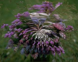
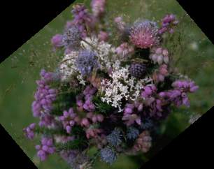
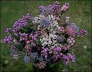
A. Appendix - images
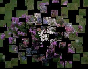
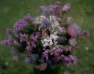
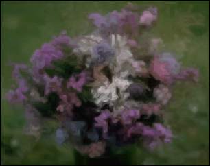
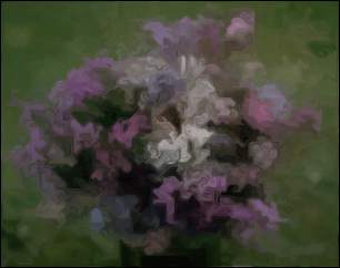
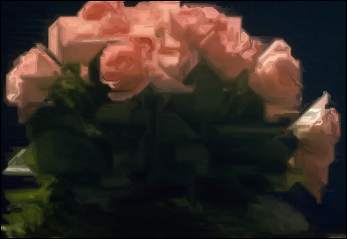
Some transformations of the image chosen will be presented.
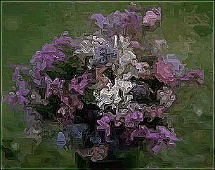
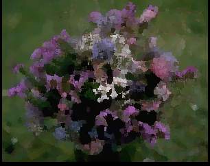
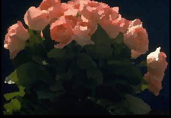
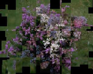
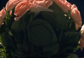
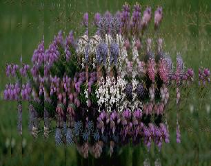
Original pictures:


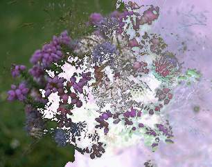
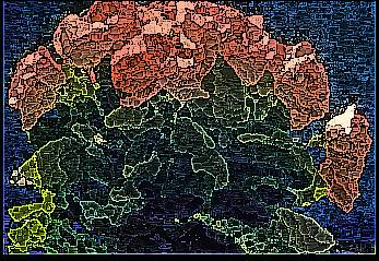
Oil painting:
|
Slice effect: |
Shear effect: |
|
Melt effect: |
Tile effect: |
|
Solarisation effect: |
Negative: |
|
Caricature: |
Fish Eye effect: |
|
Cylinder effect: |
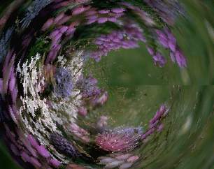
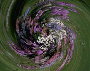
Whirlpool (swirled): |
|
Bathroom: |
Bathroom2: |
|
Rotate image (40°): |
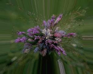
Spread effect: |

|
Pixelized image: |
Blur image: |
![]()

|
Horizontal mirror: |
Sharpen image: |
|
LIC algorithm with L = 10: |
LIC algorithm with L = 25: |
|
LIC algorithm with L = 50: |
LIC algorithm with L = 30: |
|
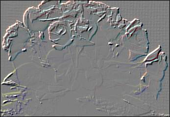
Emboss filter (Relief map): |
Filter combination Oil-painting and Sharp (99%): |
|
Oil-painting and Sharp (80%): |
LIC and Enhanced edges: |