Acoustic Simulation Techniques
In this chapter common techniques that have been implemented in different VR systems for simulation of VR scene acoustics will be presented. All of them assume that the scene description contains information about acoustical properties of all surfaces within the scene. The traditional techniques used by classical acoustics to estimate acoustic properties of real rooms using wave theory cannot be used for real time computations because of the complexity of computation. The new methods combine the knowledge of acoustics with methods developed over 30 years on the field of 3D graphics.
The Basics
Although propagation of sound waves resembles propagation of light there are important differences that affect the process of sound rendering.
Sound Velocity
The velocity of sound in air is approximately 345 m/s which is comparable with velocity of objects in our world so the Doppler shift in sound frequency is likely to happen. This is not the case with light. The equation shows how the frequency changes when a sound source has non zero velocity relatively to the listener.
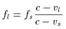 Where fl is the frequency of received sound, fs is the frequency of the sound produced by the source, vl is the velocity of the listener, vs velocity of the sound source and c the velocity of sound propagation in given media.
Sound Intensity
The air absorbs sound energy according to the equation.
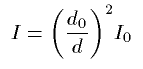 Where I is the intensity of sound in the distance d, I0 is the reference intensity measured from the distance d0.
Geometrical Methods
Image Source Method
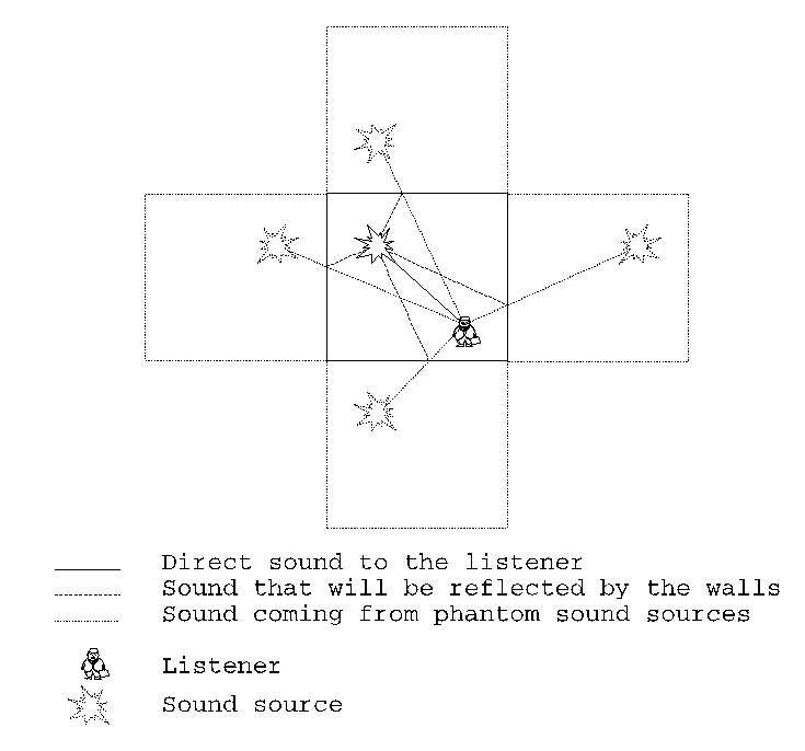 This method originates in geometrical acoustics which states that only specular reflections of sound are important. Common method is used in computer imaging for rendering of mirroring surfaces in raidosity.
The real scene is complemented with additional images of original space mirrored by walls that are to reflect the sound. The intensity of the new sound sources is decreased according to the absorption of walls and air. Only direct propagation of sound from the original source and from new sources (resulting from mirroring) is then taken in account. The number of new sound sources increases geometrically with number of reflections. In non rectangular rooms sound sources that will not be ``visible'' from the listener position must be removed from the scene.
This method originates in geometrical acoustics which states that only specular reflections of sound are important. Common method is used in computer imaging for rendering of mirroring surfaces in raidosity.
The real scene is complemented with additional images of original space mirrored by walls that are to reflect the sound. The intensity of the new sound sources is decreased according to the absorption of walls and air. Only direct propagation of sound from the original source and from new sources (resulting from mirroring) is then taken in account. The number of new sound sources increases geometrically with number of reflections. In non rectangular rooms sound sources that will not be ``visible'' from the listener position must be removed from the scene.
Particle Tracing
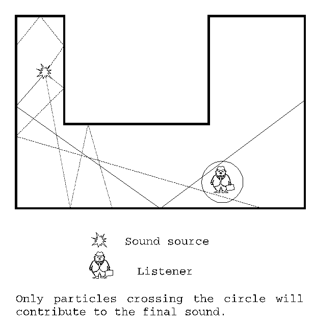 Particle tracing is basically a reverse ray tracing, which is well-known in computer graphics. Particles can be treated as small amounts of acoustical energy that are radiated from the sound source. The density of particles radiated in particular direction may be constant for the whole space or may in some way reflect the spatial characteristic of the sound source. Particles then travel through the scene while their energy will decrease due to the absorption in air and in the walls during refraction. The intensity and directional properties of sound will be obtained by summing all the particles that have reached the listener's position. If the sound source and the listener move relatively to each other, then the particles should hold information about the direction they have been radiated in. In combination with direction and velocity of the listener and the sound source the Doppler shift in frequency may be established. Restricting the direction of particles radiated from sound source according to a prediction about their way to the listener may fasten the computational time, but the results may be inaccurate especially in complex scenes.
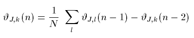
Statistical Methods
In statistical acoustics no attention is being paid to particular sound reflections. Instead of tracing the way of sound energy, statistically important characteristics of particular parts of the scene are collected to form the basis for computations. Statistical approach can be used for establishing values of reverberation time.
Reverberation Time
Energy of sound waves in the space will decrease after the sound source stops to produce sound. Time interval during which the energy drops to 10-6 of its original intensity is called the reverberation time. The reverberation time of a sound source can be considered independent of the source position. It is also independent of the listener position and the influence of an absorbing object is practically independent of the object position.
The reverberation time t of a volume V surrounded by surface of total size S is (according to Sabine)
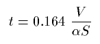
Where  is the absorption coefficient.
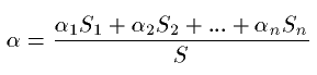
If the surface is not homogeneous then
is the absorption coefficient.
If the surface is not homogeneous then
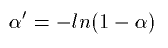
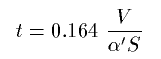
For surfaces with value near 1 t would be 0.164V/S instead of 0. To adjust this Eyring established
and
Reverberation time is good for user's judgment of character of the room he/she is in. But in fact reverberation time does not tell anything about the process of sound energy absorption in the environment. Some frequencies disappear sooner, some are present longer due to resonance (Resonant frequencies are called eigenfrequncies of the room). To reflect this fact room response function should be used rather then applying just the reverberation time.
Room Response
Room response is an impulse response of a room. Impulse response is being used for simulation or room reverberation via finite impulse response filters (FIR). Synthetic or measured impulse response of a room is applied on a sound by convolving it with the sound samples.
Room Response Measured in Real Environments
Taking samples of impulse response in a real room may significantly enhance fidelity of VR presentation even if the graphical representation is of poor quality (dark places, low detail). Even if there is a good model of room for computational simulation of room response, it cannot supply as detailed information about room acoustics as the real measurement. On the other hand additional hardware is needed to perform such measurements not mentioning the fact that VR scene does not need to be based on an existing environment.
Waveguide Mesh Method
High computational complexity of room response makes it inevitable to precompute it in advance as a part of preprocessing of the VR scene. Geometrical acoustics methods fail to yield good result for lower frequencies because they do not reflect sound waves diffractions (on lower frequencies the wavelength of sound waves is comparable to dimensions of objects within the scene). Finite element method seems to be to heavy weapon for this problem because of its complexity. A 3-D finite difference mesh (waveguide mesh) introduced in [Sav94] reduces both memory and computational complexity of that computation. Method originates in one-dimensional digital waveguides used for simulation of musical instruments. 3-D mesh simulates vibrations of air in a room.
Quoted from [Sav95]
A higher-dimensional waveguide mesh is a regular array of 1-D waveguides arranged along each perpendicular dimension, interconnected at their crossings. Two conditions must be satisfied at a lossless junction connecting lines of equal impedance: (1) the sum of inputs equals the sum of outputs (flows add to zero) and (2) the signals in each crossing waveguide are equal at the junction (continuity of impedances). Based on these difference equation can be derived for the nodes of an N-dimensional rectangular mesh:
 where
where  represents the signal pressure at a junction at time step n, k is the position of the junction to be calculated and l represents all the neighbors of k. This waveguide equation is equivalent to a difference equation derived from the Helmholtz equation by discretizing time and space.
Boundary conditions can be modeled by adding special termination nodes to the ends of each waveguide. These nodes have only one neighbor and thus behave as in 1-D waveguides. An open end with zero impedance corresponds to binding a node to zero:
represents the signal pressure at a junction at time step n, k is the position of the junction to be calculated and l represents all the neighbors of k. This waveguide equation is equivalent to a difference equation derived from the Helmholtz equation by discretizing time and space.
Boundary conditions can be modeled by adding special termination nodes to the ends of each waveguide. These nodes have only one neighbor and thus behave as in 1-D waveguides. An open end with zero impedance corresponds to binding a node to zero:
 , and produces a phase-reversing reflection. Walls that make phase-preserving reflections have an infinite impedance equation:

 . Anechoic walls would have boundaries of matched impedance corresponding to a mesh that continues to infinity. We approximate this situation with termination nodes of a one-dimensional waveguide::
 Theoretically, waves in a 3D mesh propagate through one diagonal unit in three time steps. Thus the simulation time step must be::
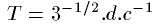 , where d is the distance between two nodes in the mesh and c is the speed of sound in the medium. For example, if d equals to 10 cm, the update frequency of the mesh is approximately 6kHz.
An inherent problem with finite difference methods is the dispersion of wavefronts. High frequency signals along the coordinate axes are delayed, whereas diagonally the waves propagate undistorted. For this reason the model is valid only at frequencies well below the update frequency of the mesh. Possibilities to reduce this effect are to use a denser mesh or higher order difference equations, which both would increase computation times.
, where d is the distance between two nodes in the mesh and c is the speed of sound in the medium. For example, if d equals to 10 cm, the update frequency of the mesh is approximately 6kHz.
An inherent problem with finite difference methods is the dispersion of wavefronts. High frequency signals along the coordinate axes are delayed, whereas diagonally the waves propagate undistorted. For this reason the model is valid only at frequencies well below the update frequency of the mesh. Possibilities to reduce this effect are to use a denser mesh or higher order difference equations, which both would increase computation times.
3D sound Output
Once all the sounds that listener can hear from its position are found and adjusted according to acoustics parameters of VR scene, an actual output should be performed that would be capable of persuading the listener that all the sound sources exist on their ``virtual'' positions. The technique of 3D sound output depends on devices used as electro-acoustic transducers.
Headphones Output - HRTF
Head related transfer function (HRTF) is mainly used for headphones as electro-acoustic transducer although attempts to use it for loudspeaker have been done (for example [Gar]).
Acoustical signal coming from different directions to a listener interacts with parts of the listener's body before it reaches eardrums in both ears. As a result of this interaction the sound reaches eardrums modified by echoes from the listener's shoulders, by interaction with the head, by the pinna response and by the resonance in the auditory canal. We can say that the body has a filtering effect on the incoming sound. Because of the speed of sound in air the significant inter-aural time delay can be noticed depending on the sound source position (in frequencies below 200Hz it is perceived as a phase shift of the sound). The sound distortion depends on sound source position (relatively to the head). The HRTF is a function of azimuth and elevation of sound source that describes the filtering effect of ``virtual user's'' body on sound coming from the given direction. For certain azimuth and elevation HRTF gives us two sets of parameter for numeric filters each for one ear. The sound that results from application of these filters on the original sound seems to the listener as if it was coming from outside of his/her head and from a particular direction.
Values for numeric filters (Finite impulse response filters for example) can be measured with a miniature probe placed near the eardrum. Impulse response of sounds that came from changing position can be then directly applied in FIR filters. There have been also successful attempts to simulate the HRTF.
HRTF of different persons varies, but an averaged HRTF of a few subject can perform well for most of the users. The best results though are achieved with ``personal'' HRTF measured on the user. The sign that a HRTF is not good for a particular user is the loss of externalization - the feeling of sound being placed outside of the head.
Loudspeaker Output
In so called virtual caves multichannel loudspeaker output is often preferred to headphones. A set of loudspeakers simulates virtual sound sources by superposing sound signals from stable mounted loudspeakers. The amplitudes of sound waves that should be produced can be calculated like this:
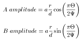 Where a is the amplitude of the virtual sound source.
This method was described in [Gar2]
Where a is the amplitude of the virtual sound source.
This method was described in [Gar2]