Previous chapter described the mathematical background of the texture mapping. No less interesting topic is creating deformed meshes in 2D. We put one important constraint on deformed surface simulation – simulation should not generate overlapping tetragons to get appropriate texture mapping. If requirement of overlapping occurs, it is possible to satisfy it by creating a several vector objects with texture mapping fill style, which overlap one another.
The most important problem is to simulate sphere surface by 2D mesh approximately, because appropriate inverse transformation from sphere surface which save proportions does not exists. Problem of cylindrical surfaces seems to be relative easy. There are several approaches to generate deformed meshes:
Maybe a brief overview of bad, better and quite good meshes should be useful to understand which kind of 2D deformed mesh is better and why.
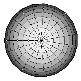
Figure 7: Bad Part of Sphere Surface – Mesh #1
In Figure 7 the projection of sphere created as rotary surface is shown. Center of the projection is intersection of many degenerated mesh cells. So, too much "covering material" is accumulated there. It is not natural effect.
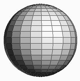
Figure 8: Better Part of Sphere Surface – Mesh #2
The middle part of the projection in Figure 8 could be a better base mesh suitable for next deforming.
Figure 9: Control points of Bézier or Beta-Spline Surface
Figure 10: Beta Spline Surface with phantom vertices can be used as 2D mesh
Figure 9 represents the control points of Beta spline surface which is rendered in Figure 10. This approach works also in 2D nicely, though these pictures are taken from our 3D spline surfaces demo. Sample points of Beta spline surface could be used to create mesh cells for texture mapping. If this approach should be used, it’s important to implement only such interaction algorithms, which allow to modify control points, but save the constraint of non-overlapping mesh cells.
Mesh #4 shown in Figure 11 is good base mesh for simulations cylindrical surfaces. Concentration of texture is realistic.
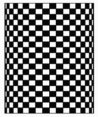
Figure 11: Quite good cylindrical mesh #3
Figure 12 demonstrates example of speculative sphere surface simulation. Sample points of square outlines are mapped on the particular circle outlines. Circles outlines are the same as in projection of Mesh #1. Number of sample points on circles is 8i, if we consider that circle with order number i=1 is the smallest non zero circle. It’s possible to see unwanted effects at diagonals especially.
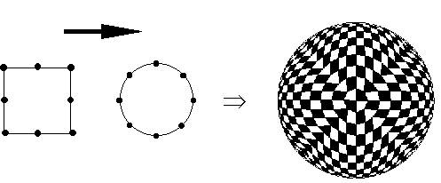
Figure 12: Bad Spherical Mesh #4 of 20 x 20 points
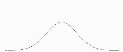
Figure 13: Gauss like curve
In Figure 13 graph of interesting function is shown. The function satisfies properties of gauss curve approximately. It’s form is:
![]()
This kind of curve is useful to influence something locally, because:
![]()
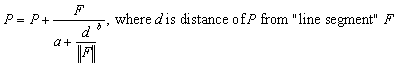
This property is used to simulate some pseudo repulsive points in mesh. All points of mesh we can transform to get the effect of repulsive point P. Point P has associated attribute which determine the pseudo power domain – power_radius. This radius determines boundary of transformation domain. The transformation of each mesh point X has form:
![]()
Coefficient a, b are arbitrary. The rather good values are about 7.0 for a and 2 for b.
We have applied this kind of transform on mesh #3. Result is mesh #5 shown in Figure 14.
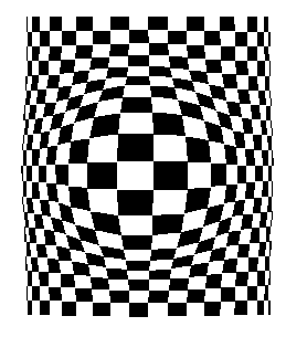
Figure 14: Combination of existing mesh #4 and pseudo sphere Ţ mesh #5
The mesh #6 (in Figure 15) has been created from mesh #5 using another special warp algorithm which is based upon the algorithm published in [Be92]. The published algorithm is based upon field morphing and it serves for warping bitmapped images. Simply said, it means that designer specifies oriented line segments in source image and then he changes their locations. The changes of the line segments locations determine deform influences for all image points. The published algorithm traverses target image and for each target pixels finds the particular source pixel to set it. Our modification consists in two points:
The main idea of weighted influences according to line segment length and distance of a mesh point from particular line segment is still the same.
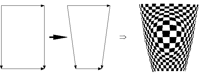
Figure 15: Deforming existing mesh #6 using warp algorithm
We develop warping algorithm simulating power influence in one point. This algorithm is based on formula:
Coefficients a, b are arbitrary. We have used 1.0 for a and 2.0 for b. Example of use of algorithm is show in Figure 16
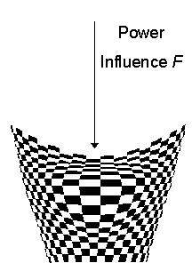
Figure 16: Mesh #7 created by power simulation from mesh #6
![]()