1. Abstract
This document tries to introduce the reader to a term derived from the word Metamorphosis, another word for transformation: Morphing.
Morphing describes the action taking place when one image (in this case a digital image) gets transformed into another or, in a more technical way, Morphing describes the combination of generalised image warping with cross-dissolve between image elements.
The idea is to specify a warp (warping, see chapter 3.2) that distorts the first image into the second.
By doing this effectively a viewer experiences the illusion that the photographed or computer generated subjects are transforming in a fluid, surrealistic, and often dramatic way.
The introduction gives a short overview over the development of morphing. This paper also introduces warping, which is the technique morphing is based on.
Four different Morphing methods, respectively related approaches are described in section 3.
2. Introduction
In the early states of Image Metamorphosis special filmmaking techniques were used, but now and since at least one decade the Morphing process is executed by computers and that in a much more convincing way.
2.1 Metamorphosis without computers
In early days morphing was dominated by the usage of cheap and not very realistic photographic effects (like cross-dissolve or fading, in which one image is faded out while another is simultaneously faded in).
Doing this as good as possible leads to the so-called stop-motion animation, in which the subject is progressively transformed and photographed one frame at a time. - But there are major disadvantages in connection with this process: doing stop-motion causes a lot of tedious work and visual strobing by not providing the motion blur normally associated with moving film subjects. Trying to fix the above mentioned disadvantages led to the so-called go-motion. Here the frame-by-frame subjects are photographed while moving. Now you get a more realistic effect by having proper motion blur, but the complexity becomes even greater due to the motion hardware and additionally required skills.
2.2 Computer Aided Metamorphosis
One great progress in morphing was the usage of computer graphics to model and render images, which transform over time.
There are two reasonable ways a computer can "see" objects (or work with objects) for transformations – 3-dimensional and 2-dimensional. Working with objects in 3-dimensional space involves a collection of polygons used for their representation. For the purpose of metamorphosis the vertices of the first object get displaced over time to coincide in position and colour of the second object (colour gets interpolated). Both objects must have the same number of polygons to allow correspondence between the vertices. Problems occur if the topologies of the two objects differ (e.g. one has got a hole through it).
In a lot of cases the manipulation of 2-dimensional images leads to the same results as doing so with 3-dimensional objects.
2.3 Morphing
Morphing is an image processing technique typically used as an animation tool for the metamorphosis from one image to another.
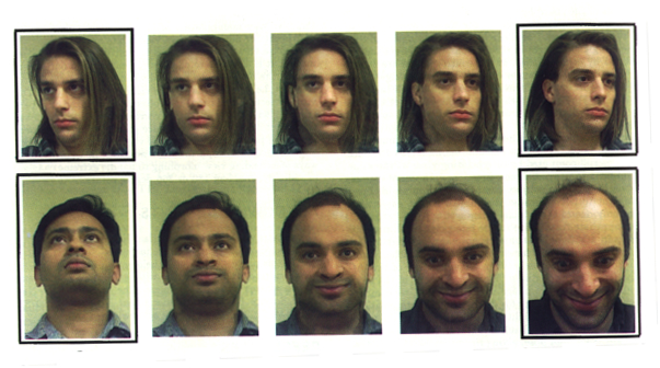
The whole metamorphosis from one image to the other consists of fading out the source image and fading in the destination image. Thus, the early images in the sequence are much like the source image and the later images are more like the destination image. The middle image of the sequence is the average of the source image distorted halfway toward the destination image and the destination image distorted halfway back to the source image. This middle image is rather important for the whole morphing process. If it looks good then probably the entire animated sequence will look good. For example, when morphing between faces, the middle "face" often looks strikingly "life-like" but is neither the first nor the second person in the image.
3. Tricky Morphing Techniques
I would like to introduce three different approaches concerning morphing.
3.1 Field Morphing
This morphing algorithm is basically based on fields of influence surrounding 2-dimensional control primitives.
In general there exist two different ways of image warping.
Forward Mapping scans through the source image pixel by pixel, and copies them to the appropriate place in the destination image. Reverse Mapping goes through the destination image pixel by pixel, and samples the correct pixel from the source image. The advantage of this algorithm is that every pixel of the destination image gets set to something appropriate. This deformation method will be used with field morphing.
Transformation with One Pair of Lines
One basic concept of field morphing consists of a pair of lines, one defined relative to the source image and the other defined relative to the destination image. These lines define a co-ordinate mapping from the destination image pixel co-ordinate X to the source image pixel co-ordinate X’ resulting in a line PQ in the destination image and P’Q’ in the source image (see figure below).
The value u is the position along the line, and v is the distance from the line. The value u goes from 0 to 1 as the pixel moves from P to Q, and is less than 0 or greater than 1 outside that range. The value v is the perpendicular distance in pixels from the line. If there is just one line pair, the transformation of the image proceeds as follows:
For each pixel X in the destination image
X’ is the location to sample the source image for the pixel at X in the destination image. The location is at a distance v (the distance from the line to the pixel in the source image) from the line P’Q’, and at a proportion u along that line.
The algorithm transforms each pixel co-ordinate by a rotation, transformation, and/or a scale, thereby transforming the whole image.
Transformation with Multiple Pairs of LinesEverybody can imagine that more than one pair of lines results in a more complex transformation. However, weighting of the co-ordinate transformations for each line has to be performed. The weight assigned to each line should be strongest when the pixel is exactly on the line, and weaker the further the pixel is from it.
In the above figure, X’ s the location to sample the source image for the pixel at X in the destination image. That location is a weighted average of the two pixel locations X1’ and X2’, computed with respect to the first and second line pair, respectively.
The closer the pixels are to a line, the more closely they follow the motion of that line, regardless of the motion of other lines.
Pixels near the lines are moved along with the lines, pixels equally far away from two lines are influenced by both of them.
Morphing Between Two Images
A morph operation blends between two images, I0 and I1. To do this, we define corresponding lines in I0 and I1. Each intermediate frame I of the metamorphosis is defined by creating a new set of line segments by interpolating the lines from their positions in I0 to the positions in I1. Both images I0 and I1 are distorted toward the position of the lines in I. These two resulting images are cross-dissolved throughout the metamorphosis, so that at the beginning the image is completely I0. Halfway through the metamorphosis it is half I0 and half I1, and at the end it is completely I1.
There are two different ways to interpolate the lines.
The first way is to just interpolate the endpoints of each line. The second way is to interpolate the centre position and orientation of each line, and interpolate the length of each line.
Advantages & Disadvantages
The probably biggest advantage of this technique is that it is very impressive and the animator is free to position the lines he wants for the image to build the reference base lines during the morphing process, corresponding from the source image to the destination image.
The two biggest disadvantages of the feature-based technique are speed and control. Because it is global, all line segments need to be referenced for every pixel, which can cause speed problems. – In some line combinations and special transformation processes unexpected and unwanted interpolations are generated, that cause additional fixing effort.
Nice Samples
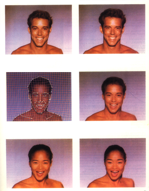
The upper left image is the upper right source
image distorted to the intermediate position.
The lower left image is the lower right destination image distorted
toward that same position.
Note that the blend (morph) between the two distorted images (middle right image)
is much more life-like than the either of the distorted images
themselves. The middle left image shows the morphed image with the interpolated lines drwan over it.
The final sequence are the images on the left side top-down viewed.
3.2 Skeleton-Based Image Warping
Image warping is a geometric transformation that maps a source image onto a target image.
In image processing, warping is used to rectify distorted images, mapping nonrectangular patches onto rectangular ones.
In computer graphics, warping plays an opposite role: the target image is the 2D projection of a 3D surface onto which the source image had been mapped. Hence warping is a composite mapping of the reparameterization from 2D image (texture) space to 3D object space, and the subsequent projection onto 2D screen space. Consequently, rectangular patches are mapped onto nonrectangular ones. This procedure is known as texture mapping.
The algorithm described in this chapter treats an image as a collection of interior layers, which are extracted in a manner similar to peeling an onion. The aim is to map a source image, S, onto a target image, T, each of whose boundaries are arbitrary. Both S and T are actually subimages, which may be extracted with any kind of segmentation method. Pixels lying in the extracted subimage are designated as foreground. The remaining pixels are assigned a background value.
The mapping will effectively treat S as if it were printed on a sheet of rubber, and stretch it to take the shape of T.
Three Stages of the Algorithm
The warping algorithm has three stages:
Reparameterize S and T using a transformation function g. This yields S’ and T’, respectively. Apply a second transformation h to map (resample) S’ onto T’. Apply an inverse mapping, g-1, to convert T’ into T, the desired result.
Reparameterization into the (u,v) Parameter Space
This chapter describes the above-mentioned function of the first stage that transforms images S and T into a new parameter space. This reparameterization corresponds to function g in the above figure. The algorithm decomposes a 2D image into an alternate representation consisting of layers of interior pixels. The layers are extracted in a manner like peeling an onion. This imposes a (u,v) parameterization in which u runs along the boundary, and v runs radially inward across successive interior layers.
Since the mapping information is only defined along the boundary, it is reasonable to first consider the mapping of adjacent points. These points consist of the adjacent layer. This data can then propagate further until the innermost layer is assigned a correspondence (skeleton).
In a convex shape, an eroding boundary coincides with shrinking (scaling down) the boundary positions about the centroid (area around the centre).
Problems can arise if scaling is applied to shapes containing concavities. The reduced boundary does not lie entirely within the larger adjacent boundary, and the centroid is no longer guaranteed to lie within the shape.
The difficulty of expressing erosion analytically for shapes containing concavities is bypassed with a discrete approximation – a thinning algorithm.
Thinning
Thinning, together with boundary traversal, is used to erode foreground pixels along the boundary while satisfying a necessary connectivity constraint. This helps to impose the (u,v) co-ordinate system upon the S and T images.
Classical thinning algorithms operate on binary raster images. They scan the image with a window, labelling all foreground pixels lying along the boundary with one of two labels, DEL or SKL.
DEL is designated to set the foreground pixel as deleteable (flip to background value), if the foreground pixel is not found essential in preserving the mutual connectivity.
The SKL label is applied to skeletal points, pixels, which must be kept in order to preserve neighbourhood connectivity. This pixel is said to lie on the shape’s symmetric axis, or skeleton, which has the property of being fully connected.
After each thinning pass a boundary traversal follows.
Boundary traversal
During the Boundary traversal the boundaries are traversed while concurrently initialising the appropriate layer list (list of the appropriate image used to store the layers pixel (-colour)) and deleting those pixels labelled DEL.
SKL pixels remain intact and are guaranteed to appear in all subsequent layers.
The starting point for such a traversal is initially chosen to be the top-leftmost boundary point or a boundary point of high curvature (this decision has a bunch of advantages). – Clearly the most reliable choice for a starting point is one which is known to be contained in all subsequent layers. Since skeletal points fulfil this property, the first encountered skeletal point may be chosen to take on this role. All subsequent traversals will then begin from that skeletal point.
Example:
|
|
0/34 | 0/33 | 0/32 | 0/31 | ||||||||
| 0/02 | 0/01 |
1/00 |
1/28 | 1/27 | 0/30 | |||||||
| 0/04 | 0/03 | 1/02 | 1/01 | 2/10 | 1/26 | 0/29 | ||||||
| 0/05 | 1/04 | 1/03 | 2/12 | 2/11 | 2/09 | 1/25 | 0/28 | |||||
| 0/06 | 1/05 | 2/14 | 2/13 | 3/12 | 3/09 | 2/08 | 1/24 | 0/27 | ||||
| 0/07 | 1/06 | 2/15 | 3/13 | 4/12 | 4/08 | 3/08 | 2/07 | 1/13 | 0/26 | |||
| 0/08 | 1/07 | 2/16 | 3/14 | 4/07 | 3/07 | 2/06 | 1/22 | 0/25 | ||||
| 0/09 | 1/08 | 2/17 | 3/06 (06) |
2/05 | 1/21 | 0/24 | ||||||
| 0/10 | 1/09 | 2/18 | 2/19 (05) |
2/04 | 1/20 | 0/23 | ||||||
| 0/11 | 1/10 | 1/11 | 2/20 (04) |
2/03 (03) |
1/19 | 0/22 | 0/21 | |||||
| 0/12 | 0/13 | 1/12 | 1/13 | 1/14 (00) |
1/18 | 0/20 | ||||||
| 0/14 | 0/15 | 1/15 | 1/16 (01) |
1/17 | 0/19 | |||||||
| 0/16 | 0/17 | 0/18 |
Consider the shape given in the figure above. All foreground pixels are labled with a number (label/pos) and all skeletal pixels are highlighted with a darker background. The shape is processed in passes consisting of the following two steps each:
Apply one pass of a thinning process to label all boundary points as deleteable (DEL) or skeletal (SKL). Traverse the boundary as described in "Boundary traversal". This procedure serves to initialize the appropriate layer list and expose interior layers so that they may become traversed in subsequent passes.
Data Structure: Layer-Trees
The recursive subdivision of layers gives rise to a tree representation. A L-Tree has the following simple properties:
Each level of the tree corresponds to an interior layer of the shape, starting with the outermost layer in the root. The vertices in each level include DEL and "first-generation" SKL labelled pixels. The leaves build a strip which have no descendants, the entire strip maps onto an "old" SKL segment in the previous (upper) layer.
The internal structure of an L-Tree can be encoded as shown below:
struct {
unsigned char *imgbf; /* pointer to list */
int len; /* length of list */
int *links; /* pointer to auxiliary data */
}
The (u,v) Parameters
The (u,v) parameterisation is conveniently represented by L-Trees where the (u,v)-co-ordinates are indices into the layer lists stored in the tree vertices.
The v value corresponds to the layer beginning at the root where v=0 and the v-co-ordinate gets incremented at each successive tree level.
The u value corresponds to the layer length (number of pixels presented in each boundary).
For the following mapping within the (u,v) parameter space an image of conventional format is required, including the pixels currently stored in the L-Tree.
Mapping within the (u,v) parameter space
This section describes the function h that resamples S’ onto T’. The mapping solution in the (u,v) space is now more tractable than its counterpart in the rectilinear co-ordinate system.
First pass: normalising the v-axis
For each u resample the column of pixels along the v-axis
so that the maximum v samples are used for the corresponding radial
path (column on figure above). This forces all columns to be supersampled
at a rate dictated by the maximum v. Second pass: resampling the
u-axis
This is a similar procedure as the above normalisation; now the u-axis
in S’ gets scaled to match the dimension of T’. Third pass:
resampling the v-axis
Now that the (u,v) parameter spaces for S and T have
identical dimensions in the u-direction, the information in the
v-direction must be made identical as well – column by column.
Reparameterization from (u,v) to (x,y)
Now the resampled data of S’ has to get reapplied onto T, corresponding to the function g-1. Two steps are required (reverse procedure of "Reparameterization into the (u,v) Parameter Space"!):
Scale the appropriate intervals along the row of T’ to update the layers in T’s L-Tree (by using interpolation). Traverse shape T while concurrently updating the traversed pixels with the values stored in the L-Tree.
Advantages & Disadvantages
The algorithm described is an efficient way to perform image warping among arbitrary shapes.
In spite of not being the most effective algorithm the described approach equipped with a few extensions from the current discrete implementation to a continuous domain offers promising possibilities for increased accuracy and control.
A few examples
The following two figures show how images can be mapped onto arbitrary shapes:
The first figure shows four images. S and T are displayed in the upper left and lower left quadrants, respectively. The lower right quadrant shows S mapped onto the shape defined by the foreground pixels of T. The mapping of T onto S is shown in the upper right quadrant.
This figure shows two textures mapped to the target facial shape (the second texture is the chess board of the figure above).
3.3 View Morphing
This part of "Tricky Morphing Techniques" introduces a simple but very challenging extension to image morphing that correctly handles 3D projective camera and scene transformations.
Introduction
Because no knowledge of 3D shape is required, the technique may be applied to photographs and drawings, as well as rendered scenes.
View morphing between two images of an object taken from two different viewpoints produces the illusion of physically moving virtual camera. The effect can be described by what you would see if you physically moved the object (or the camera) between its configurations in the two images and filmed the transition:
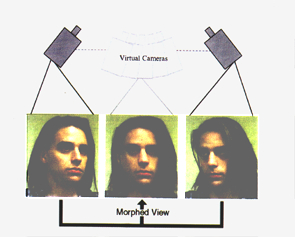
When morphing between different views of an object or scene, the technique produces new views of the same scene, ensuring a realistic image transition.
View morphing takes advantage of existing image morphing techniques, already in widespread use, for part of the computation. Existing image morphing tools may be easily extended to produce view morphs by adding the image prewarping and postwarping steps.
View morphing works by prewarping two images, computing a morph (image warp and cross-dissolve) between the prewarped images, and then postwarping each interpolated in-between image produced by the morph. The prewarping step is performed automatically while the postwarping procedure may be interactively controlled by means of a small number of user-specified control points.
Technique
Computing the morph requires the following:
Two images I0 and I1 representing views of the same 3D object or scene Their respective projection matrices M0 and M1 A correspondence between pixels in the two images
There is no a priori knowledge of 3D-shape information needed.
When the pixel correspondence is correct, the methods described in this section guarantee shape preserving morphs.
The three stages of the algorithm are:
Enhancements
The technique described in the previous chapter can be extended to accommodate a range of 3D shape deformations. View morphing can be used to interpolate between images of different 3D projective transformations of the same object, generating new images of the same object, projectively transformed.
The advantage of using view morphing in this context is that salient features such as lines and conic shapes are preserved during the course of the transformation from the first image to the second.
Another enhancement is to leave out the prewarp entirely in cases of considerably different objects. Prewarping is less effective for morphs between different objects not closely related by a 3D projective transform. - The postwarp step should not be omitted, however, since it can be used to reduce image plane distortions for more natural morphs.
Advantages & Disadvantages
Because no knowledge of 3D shape is required, the technique may be applied to photographs and drawings, as well as to artificially rendered scenes. This is probably the most remarkable advantage of view morphing.
Since view morphing relies exclusively on image information, it is sensitive to changes in visibility. Problems occur if the visibility is not constant, i.e., not all surfaces are visible in both images. A related problem that has not been solved yet is the usage of view morphing for 180° or 360° rotations in depth.
Nice Samples
4. Conclusions
The morphing techniques introduced in this document have one thing in
common: they concentrate on a topic of computer graphics, which is one
of the most fascinating aspects of computer graphics.
The papers that this document is based on are only a subset of morphing
techniques and closely related computer graphics applications.
One of the early useful morphing techniques, skeleton-based image warping by Georg Wolberg, involved an interesting way to map a 2-dimensional image to an arbitrary shape.
Using this morphing technique as a starting point, Thaddeus Beier and Shawn Neely developed a challenging morphing technique for transforming one digital image into another by giving the animator high-level control of the visual effect, such as natural feature-based specification and interaction.
Finally, view morphing (Steven M. Seitz and Charles R. Dyer.) extended both of the techniques above to artificially create realistic "in-between views" of an object (or two similar objects) as 2-dimensional images taken from two different viewpoints.
I hope I succeeded in catching your attention with my computer graphic approach to the latest morphing techniques.
5. References
Thaddeus Beier, And Shawn Neely, "Feature-Based Image Metamorphosis"
Georg Wolberg, "Skeleton-based image warping"
The Visual Computer 1989. pp. 95-108.
Steven M. Seitz, And Charles R. Dyer, "View Morphing"
Proc. SIGGRAPH 96. In Computer Graphics (1996) pp. 21-30.