2. Data structures

I now want to describe some of the basic data structure we used for our library.

2.1. Tree structure

We use a tree to represent the scene we want to render. The tree structure we use is very similar to the trees used by openInventor or Performer[2].

Basically there are two types of nodes in our tree:

• transformation nodes
• object nodes

Transformation nodes basically are good old 4x4 transformation matrixes, describing the movement of the object nodes 'below' the transformation nodes.

Object nodes are some sort of movable objects - usually geometric objects, cameras, lights and so on.

When we want to render the scene, we initialize a transformation matrix with the identity matrix. Then we recursively traverse the tree. Each time we meet a transformation matrix we combine this transformation with our current transformation matrix (simple matrix multiplication).

Each object node we meet, we transform with the current transformation matrix. Whenever we return from a sub-tree we have to restore the original matrix. This can easily be achieved by the use of a matrix stack.

Because transformation matrixes are combined while we go down in our tree, we have a very natural way to describe geometric dependencies.

Lets look at an example scene with a light and a car with its four wheels:

 



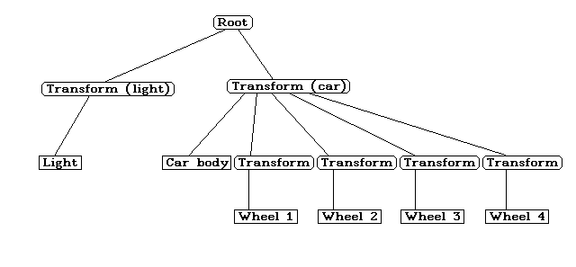
Fig. 1: the scene tree

In the scene described in Fig. 1 there's a transformation matrix for the light and for the car. This means that the light and the car can move independently from each other.

The car transform has five 'children': The car body, and 4 transforms, each for one wheel of the car.

Because the wheel transforms are combined with the car transforms, the wheels can have their individual movement (spin, etc.) and still also have the same overall movement of the car. So if the car moves to the left, all four wheels do the same left movement as the car body, plus their individual movement.

Summary: The whole scene is kept in a tree. There are two basic nodes: 'transforms' and 'objects'. 'transforms' are combined as we traverse the tree and are applied to 'objects' below them in the tree. 'objects' can be anything from lights to cameras, to geometric data.

2.2. The 'transform' Object

The 'transform' structure is a class which is derived from the class 'node' which is our basic tree handling object. 'node' has a few basic functions to manage the handling of children and parents of a node in the tree.

'transform' uses the following variables: (and some more)

center // center of rotation scale // scale factor for x, y, z translation // translation orientation (heading, pitch, roll) // rotation a'la airplane rotation // rotation around a free axis matrix // the resulting 4x4 matrix invertedMatrix // the inverted matrix

Each of the components (center, scale, etc.) are private member variables and have to be set by a special setXXX procedure. For example:

void setCenter (vector3 _center) // set rotation center vector3 getCenter (void) // get rotation center

Although it's possible to set the whole transformation at once ( void setMat (matrix _m) ) it's highly recommended to use the different setXXX functions to 'construct' the matrix you want.

Usually that's easier for the user anyway. And besides it gives us the chance to keep track of the kind of the matrix.

It's quite common that one only needs a simple translation matrix. E.g. to place a object in the scene. In this case, the user should call setTranslation (xxx). Transform then sets an internal variable indicating that this transform uses a translation.

If other transformations (rotations, scales) are used too, 'transform' keeps track of those too.

So, when it comes to using the transform, we know how the matrix is structured, and with a little luck we can save some processing time using that knowledge:

When we traverse the tree and have to combine two matrixes, and one of the two is for example a translation matrix, we don't have to do a full matrix multiplication. In the best case we only have to add the translation factors.

In that case we would have a drastic performance gain: 3 float adds instead of 64 float mul's for a full blown matrix multiplication!

Knowledge of the matrix structure also can be very handy when we need to calculate the inverted matrix.

And finally, the setScale function also checks whether it's an uniform scale or a non uniform scale. This is no concern when multiplying matrices, but it's useful information when doing light calculations.

As long as it's a uniform scale, our normal vectors don't have to be re-normalized, which too can be quite a time saver.

Summary: Try to get as much information about your transformation matrix so you can do the following optimizations:

• do 'smart' matrix multiplications
• do 'smart' inverse calculations
• keep track of non-uniform scales

2.3. The 'geode' Object

The class 'geode' holds any form of geometric data. A 'geode' is what sometimes is called an graphics object.

Typical examples for geodes are simple graphical objects like cubes or spheres, or the model of a house and so on. Since 'geode' is derived from 'node' it is a part of our tree structure.

In the above example Car body and Wheel 1 to Wheel 4 all where 'geodes'.

Geodes can be very simple, a single cube for example, but they can also be very big and complicated like a complete VRML-world with hundreds of thousands of vertices.

The only restriction a 'geode' has to obey is that it has to be static in itself. That means that no part of a geode can have a different movement than any other part of a geode.

This is because each part of the 'geode' is transformed with the same 'transform' object. This is the reason why we had 4 independent geodes for the wheels in our above example - so that the wheels can move independently from the car body. However the whole car still has a common movement because all 5 geodes have one common 'transform' object to them.

Summary: A 'geode' is a set of geometric data which has a common movement. If you want to build 'logical movement groups' like the car « wheel or human body « arm « hand « finger grouping, you have to do that at the tree level instead at 'geode' level.

2.4. The 'geoState' Object

The class 'geoState' describes the appearance of geometric data. A 'geoState' can be thought of as a material description. It includes:

texture // which texture map to apply frontmaterial // the material for 'front' faces // material = ambient, diffuse, specular coeff., // emissive color, attenuation, etc. backmaterial // material for 'back' faces fog // fog definition (linear, exponential, per vertex, per pixel) culling mode // cull clockwise or counterclockwise shading mode // flat shading or gouraud shading lights // list of active lights

most of the variables of a 'geoState' are again specialized classes. 'texture' for example is a class of it's own with many parameters, e.g. type of filtering, type of mip-mapping, texture format, size, detail textures, etc.

The basic idea of a 'geoState' is to fully describe the state of the rendering pipe. Whenever we want to render faces with the properties of a 'geoState' we apply it. The apply function calls the appropriate functions of the underlying rendering API, thus setting the rendering state to that of our 'geoState'. All polygons rendered after this call will use the texture, lights, fog, material and so on defined by the 'geoState'.

A little bit later we will discuss the topic of state switching / state setting in more detail.

Summary: A 'geoState' fully describes the appearance of geometric data. To set the rendering state according to a 'geoState', the apply function is called.

2.5. The 'geoSetPoly' Object

The class 'geoSetPoly' holds geometric data - just like a geode. But with one difference: a 'geoSetPoly' only holds geometric data of the same type.

In fact each 'geode' is built of one or more 'geoSetPoly's. A 'geode' is only a container for different 'geoSetPoly's.

(For a full description of the geode - geoset - geostate idea, see [2] )

To give you a fast picture before going into detail, let's imagine we want to describe a wooden table with metal feet.

We use two textures: a wooden texture and a metal texture. In that case the table would be a 'geode' which would consist of two 'geoSetPoly's. The first 'geoSetPoly' would hold all faces which use the wood texture, the second 'geoSetPoly' would hold all faces which use the metal texture.

Earlier I said that a 'geoSetPoly' holds geometric data of the same type. In our case having 'the same type' means to have the same 'geoState'. As said before a 'geoState' can be thought of as a material of some kind. For each material we need in a scene, we have to define a 'geoState'. All geometric data (= 'geoSetPoly') of that material has a pointer to the 'geoState' representing the material.

So many different 'geoSetPoly's might use the same 'geoState'.

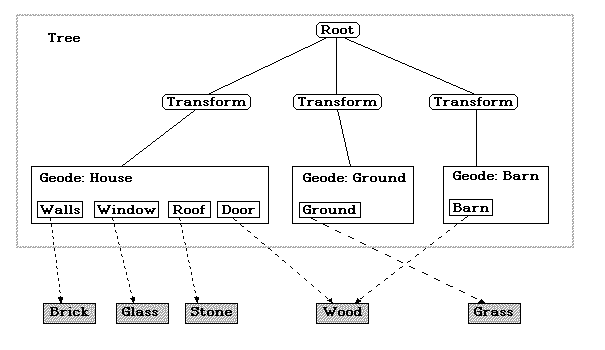
Lets look at an example of a brick house with a wooden door, glass windows, and a stone roof. (Fig. 2) The house is placed on a grass ground, and next to the house is a wooden barn. Our scene tree would look like this:



Fig. 2: a scene showing the dependencies of geode « geoSetPoly and geoSetPoly « geoState

There are a few things one should notice in the above illustration (Fig. 2):

• Each 'geode' has an own transform node. That's not necessary. If all geodes would use the same coordinate system, they could all use the same 'transform'.
• Each 'geode' consists of at least one 'geoSetPoly'. A geode that needs only one material has only one 'geoSetPoly', a geode that needs several materials has several 'geoSetPoly's, one for each material.
• Each 'geoSetPoly' has one 'geoState'.
• 'geoState's can (have to) be shared among 'geoSetPoly's.
• transforms are applied to whole 'geode's, not to independent 'geoSetPoly's

Summary: Each 'geode' is split into several 'geoSetPoly's for each 'geoSetPoly' has a 'geoState'. 'geoState's can be shared.

3. Optimizing state switches

Now one might ask: Why do all this? Why do we have to split a 'geode' into several 'geoSetPoly's? The answer is: to minimize state switches of the rendering pipeline.

A state switch is what happens when a 'geoState' is applied (= made active). We mentioned that already earlier. But what we didn't say is, that a state switch can be an extremely costly operation, which takes very long to execute.

There are many state variables that have to been set, and often the setting of a simple state variable causes many internal operations in the rendering API (loading of different fog table, for example) which can take extra time.

(In fact, most rendering API's are implemented as 'state machines', which makes optimized state switches particularly interesting. For an explanation of the state machine concept, see OpenGL - [1])

But probably the most important thing is the switch of the current texture map. The switching between two texture maps can take amazingly long on some systems. But even if only the switching between to textures (set the image pointers, get the current size, apply the filtering, etc.) is a fast operation on your system, there's still one big danger to texture switching: you might be out of texture memory! In that case you have to free some space in texture memory (= release a previously loaded texture) and download the texture you want to apply to the texture memory.

Let's look at an example: Let's suppose we have a textured scene of 100 'geode's, each texture is 256 x 256 x 32 bit (RGBA) with all mip mapping levels. Let's suppose further that while drawing each geode we have to do 1 texture download (that's an optimistic guess!!). In that case, each frame, we would have the following memory transfer:

100 x 256 x 256 x 4 x 1.333 (mip maps) = 33 megabytes. Each frame. This would simply be too much for today's PC systems memory transfer rates.

So what we do is this: we sort the 'geoSetPoly's by their 'geoState'. When drawing, we apply the first 'geoState', then draw all 'geoSetPoly's that use that 'geoState', then apply the next 'geoState', draw it's 'geoSetPoly's, and so on.

As a secondary sort criteria we use the texture of the 'geoState'. So if there are 'geoState's which use the same texture, but different, for example, front materials, they would be neighbors after sorting.

That way we minimize the most costly texture switches. As an additional optimization we keep track of the current rendering state, and when a 'geoState' is applied it only sets those variables, textures, etc. that differ from the current state. So if 'geoState' 1 enables fog and 'geoState' 2 wants fog too, 'geoState' leaves the fog variables untouched.

These two concepts are the key principles of our library:

• sort by 'geoState's
• do minimized state switch (update differences only)

It's really amazing how much time you can save by using these simple and logical principles. Of course you could always be lucky and have enough texture memory, but that's unlikely. Especially on PC based systems.

We did some testing and found out that the minimized state switch (excluding textures) can save between 5% and 10% of execution time.

The optimized switching of textures can do huge savings. We've seen cases where the performance jumped from 2 to 3 frames per second to 30 to 40 frames per second. Just because of optimized texture switches.

Summary: State switches are costly. Especially the switching between textures can take a long time. Therefor try to minimize state switches by sorting by 'geoState's and then do a minimal (delta) state update. Everything you don't do because it's already done saves precious time!

4. Display Optimizations

The following points are very simple optimizations, which can save loads of time, but still often are simply not done .

4.1. Cull faces

It's dead simple. Use backface culling. (for an explanation on backface culling see [3] ) It will save a lot of time not to draw the faces you won't see anyway.

Especially on systems without hardware z-buffering and hardware texturing it's highly recommended to use backface culling. In good cases it halves the amount of faces you have to process.

Most API's like OpenGL [1] support backface culling. However we found out that it sometimes can be useful to do the culling yourself. Because if we do it on our own, we can check if the face is visible or not, and only if it is, really send it to the API.

In the other case (the API does the culling) we have to send the full specification of the face (vertex colors, texture coordinates, vertex normals) to the API, just to let the API find out that it wouldn't have needed the information anyway, because the face is invisible.

Summary: Do use backface culling.

4.2. Cull objects (geodes)

The idea is to find out if whole geodes, or at least geoSets are out of the current field of view. If that is the case, we don't have to draw these objects.

Therefore, each 'geode' and each 'geoSetPoly' has a bounding box. The bounding box is calculated in the objects local coordinate system, and consist of two vector3 variables:

BboxMin = ( min. (all x Values), min. (all y Values), min. (all z Values))

BboxMax = (max. (all x Values), max. (all y Values), max. (all z Values))

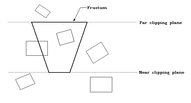
When we traverse the tree to draw the scene, we first transform each bounding box to see if the bounding box intersects the viewing frustum. The bounding box is completely out of the field of view, if all 8 vertices of the bounding box lie on the outside of at least one plane of the viewing frustum.

In all other cases, the bounding box intersects the frustum, and thus parts of the object inside the box might be visible.



Fig. 3 : a 2D view of the viewing frustum and geode-bounding-Boxes

But we only have to transform and test 8 vertices, to find out if we have to transform the whole object! If a bounding box lies entirely outside the field of view, the vertices inside the box (which might be hundreds or thousands of vertices) are not rotated, projected, etc.

In our case we first test the bounding box of the geode. If it's on the outside, all the geoSetPoly bounding boxes will be outside, too. If not, we test the bounding boxes of the geoSetPolys.

Figure 3 shows a typical scene: most bounding boxes lie entirely outside the frustum. Only very few lie inside or intersect the frustum. The test if a box intersects or not is very simple: simply 'clip' the bounding box in homogenous coordinates. [3]

This simple trick can be a huge time saver: In a usual scene, about half the objects will be in front of the near clipping plane and half the objects will be behind the near clipping plane.

In that case we only have to care about half our geodes! The far, left , right, bottom and top clipping plane reduces the amount of objects to draw even further. Roughly you could say: The larger the scene gets, the more you save!

Summary: Calculate a bounding box for each object. Before transforming the entire object first transform the bounding box, and check if its visible (intersecting the frustum) or not. Only if it's visible, transform the whole object.

5. Conclusion

All the methods we mentioned and discussed in this paper are very simple and easy to understand. They don't use complicated math or complex algorithms either. But still they are very powerful and effective methods to save time, when doing real-time graphics.

And I really believe, that this is the way to go: sit down and think, and do a little bit of optimizing, before you go out and buy an extra CPU because your program runs too slow. This way is much the cheaper, and quite often also the better way.

References

[1] Neider, Davis, Woo: OpenGL Programming Guide, Addison-Wesley Publishing company

[2] Iris Performer Programming Guide, Silicon Graphics Computer Systems, Doc# 007-1680-020

[3] Foley, van Dam, Feiner, Hughes: Computer Graphics: principles and practice, Addison-Wesley Publishing company

If you have any comments, questions or suggestions:

Erik Pojar - erik@reality2.com