An experimental system
for reconstructing a scene from the image sequences produced by a moving
camera
Jiri Walder,
jiri.walder.fei@vsb.cz
Technical University of Ostrava
Ostrava / Czech Republic
Abstract
In this paper, a method and an experimental computer
program for reconstructing a three-dimensional static scene from the sequence
of images produced by a moving camera are presented. A method for determining
the camera trajectory and for reconstructing the coordinates of feature
points from multiple images is proposed. The efficiency and the robustness
of this method are verified experimentally. The feature points and the
correspondence relation are detected automatically by a heuristic algorithm.
Keywords: scene reconstruction,
camera calibration, image processing, computer vision, point tracking.
1. Introduction
The paper focuses on the following problem: Consider
a three-dimensional static world that will be referred to as a scene.
A camera moving in this world produces a sequence of images called frames.
The frames are two-dimensional pixel arrays. The two-dimensional coordinates
of points can be measured in the frames. The sequence of the frames is
used to create a model of the scene. The three-dimensional coordinates
(in a global reference system) of the feature points that are visible in
the frames are computed.
The solution to the problem of reconstructing a scene
from a pair of stereo images is known for a long time [5]. The reconstruction
from three and multiple images was later studied from various viewpoints
[4][6]. The difficult problem involved in reconstruction is to detect the
correspondence (we say that in different frames, the images of a unique
point of a scene correspond to one another). Finding the correspondence
by a computer algorithm is hard: (1) In order to achieve a good accuracy
of reconstruction, the images should be taken from camera positions that
are distant enough. (2) As the distance between the camera positions increases,
the images become more and more different and the correspondence is more
and more difficult to find automatically. If a whole sequence of frames
produced by a moving camera is available, the problem becomes easier. Since
the change between two consecutive frames is usually small, the correspondence
relation for the consecutive frames can be found easily. Also, the effects
of occluding can be detected reliably. The correspondence relation for
non-consecutive frames can be determined as the product of the relations
for the consecutive frames. We suppose that the sequence of frames is long
enough. From this sequence, a certain set of significant frames can be
chosen for reconstruction.
In this paper, a method and an experimental computer
program for reconstructing a scene from the sequence of images produced
by a moving camera are presented. A method for determining the camera trajectory
(i.e., for calibrating the camera) and for reconstructing the coordinates
of points of interest from multiple images is proposed. The system performing
the scene reconstruction consists of the following parts: (1) Detecting
the points of interest in the particular frames. (2) Tracking the points
in the sequence of frames. (3) Determining the camera trajectory. (4) Reconstructing
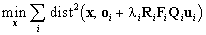
the coordinates of the points of interest. Figure 1 shows the block scheme
of the system.
The paper is organised as follows: In Section 2,
the model of the camera and camera motion is described. The method for
calibrating the camera and the method for reconstructing the coordinates
of points are presented in Sections 3.1 and 3.2, respectively. In Sections
3.3 and 3.4, the problems of detecting and tracking the points of interest
are discussed.
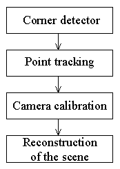
Figure 1. The block scheme of the system.
2. The model of the camera
The camera model considered is the classical pinhole
model. The basic assumption is that the relationship between the world
coordinates and the pixel coordinates is linear projective. We suppose
that the possible non-linear distortions of the images are corrected in
advance, before the images are used for calibration and for reconstruction.
As the camera moves in a three-dimensional scene, it produces a sequence
of frames. We suppose that the sequence I0,I1,...,In
of significant frames taken in times t0,t1,...,tn
is available for calibration and for reconstruction. The sequence need
not include all the frames produced by the camera. Instead, we may wait
until the changes in the frames are large enough to give new information.
The information in the dropped frames is then used indirectly (Section
3.3). Let (O,x,y,z) be a global coordinate
system in the scene (Figure 2). For each ti,
a camera coordinate system (Oi,xi,yi,zi)
is considered (Oi is the centre of projection,
zi
is the optical axis of the camera). Let
X be a point in the scene,
let x=(x,y,z)T and xi=(xi,yi,zi)T
represent X in (O,x,y,z) and (Oi,xi,yi,zi),
respectively. We have
 , ,
|
(1)
|
where Ri describes
the rotation of (Oi,xi,yi,zi)
into (O,x,y,z), and oi
represents Oi in (O,x,y,z).
We define Ri,j,bi,j
such that
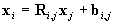 . .
|
(2)
|
Obviously, Ri,i=I
(unit matrix), and bi,i=0.
It is easy to see that (we consider
i<j and we define )
)
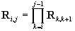 , ,
|
(3)
|
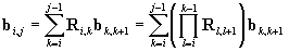 . .
|
(4)
|
Recall that Ri,j
is an orthonormal matrix and that Ri,j =Rxi,jRyi,jRzi,j.
Rxi,j,Ryi,j,Rzi,j
are the matrices corresponding to the rotations around the xj,yj
and zj-axis, respectively. We introduce the
vector ji,j
= (jxi,j,
jyi,j,
jzi,j)T
containing the rotation angles. Let fi = dist(Oi,Oi')
be the focal length of the camera in ti. In
each significant frame, we introduce a coordinate system (Oi',xi',yi')
(Figure 2). The image coordinates are measured in a coordinate system (Zi,ui,vi).
Let Xi be the image of X in the ith
frame, and let ui=(ui,vi,1)T
represent Xi in (Zi,ui,vi).
In (Oi',xi',yi'),
Xi
is
represented by Qiui
where Qi describes the transformation
of (Zi,ui,vi)
into (Oi',xi',yi').
It follows that
 , ,
|
(5)
|
where
 , ,  . .
|
(6)
|
The values u0i,
v0i
are the coordinates (in (Zi,ui,vi))
of the point in which the optical axis pierces the projection plane. The
angle qi
models a possible deviation from orthogonality of the cell array of the
sensor or a possible misalignment of the projection plane with respect
to the optical axis. In practice, qi
is usually close to p/2.
The scaling factor si takes into account the
possibly different sizes of the sensor cells along the u and
v-axis
and the distortion introduced by the frame grabber; li
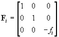
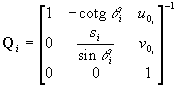
is a real parameter. The parameters in Fi,
Qi
(fi,
u0i,
v0i,
qi,
si)
are the camera intrinsic parameters. The parameters describing the trajectory
of the camera in space (Ri,oi
or Ri,i+1,bi,i+1)
are the extrinsic parameters.
3. The description of the system parts
3.1 Camera calibration
The purpose of camera calibration is to determine the intrinsic and the
extrinsic parameters of the camera. Once these parameters are known, three-dimensional
information can be inferred from two-dimensional images and vice versa.
The calibration method proposed in this paper focuses on the problem of
finding the extrinsic parameters. Thus, we suppose that Fi,Qi
are known for each i. Note that a variety of methods for determining
the camera intrinsic parameters were presented [3].
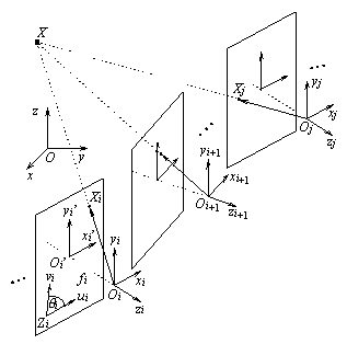
Figure 1. The model of the camera and camera motion.
The information needed for calibration is provided
by detecting and tracking the points of interest (Sections 3.3,3.4). In
this section, we suppose that from the significant frames I0,I1,...,In,
the lists of the points of interest along with their image coordinates
and along with the description of the correspondence relation can be obtained.
From the set of the pairs of corresponding points of interest, reliable
pairs are chosen for calibration. Consider two different values ti,
tj
(i<j) and a point X in the scene. Let pi,
pj
represent the directions of lines
áOiXiñ
and
áOjXjñ,
respectively, in (Oi,xi,yi,zi).
Since áOiXiñ,
OjXjñ,áOiOjñ,
are coplanar, the condition pi×(bi,j´pj)=0
must be satisfied. The conditions yields [1]
 . .
|
(7)
|
Let s = (bT0,1,
jT0,1,
bT1,2, jT1,2,
... , bTn-1,n,
jTn-1,n)T
be the vector of the values that are to be found during the calibration.
Let q be the number of calibration points, let X(k)
be the kth such point. We use u(k)
to denote the vector of coordinates of the images of X(k)
in all the frames in which X(k)
is used for calibration, and, finally, we introduce the vector u
= (u(1)T,
,u(q)T
)T
of the image coordinates of all the calibration points. The coplanarity
equation Eq.(7) can be rewritten as follows
 . .
|
(8)
|
Usually, much more points than is the minimum required
for calibration are detected in the frames. This can be used to reduce
the influence of noise, i.e., the fact that the coordinates in the frames
are measured with an error can be taken into account. Let u contain
the exact coordinates. We use u0 to denote
the vector of coordinates observed in the frames, and we introduce the
vector Du=u-u0
of the differences and a diagonal matrix W expressing the reliability
of the particular observations. The vector s then can be found by
minimising the value
 . .
|
(9)
|
The following coplanarity equations must be satisfied
 . .
|
(10)
|
We solve the non-linear problem formulated by Eqs.(9),
(10) by linearisation. Suppose that an initial estimation s0
of s is known. Let Ds
be the correction of s0, i.e., s=s0
+Ds.
By the Taylor expansion of Eq.(10), neglecting the higher order terms,
we obtain
 , ,
|
(11)
|
where
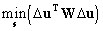
The minimisation in Eq.(9) with the condition in Eq.(11) may be solved
using the method of Lagrange multipliers. Let m
be the vector of Lagrange multipliers. The problem is solved by minimising
the function
 . .
|
(13)
|
The computation yields the result
 . .
|
(14)
|
We use Eq.(14) in the iterative process. In each step of this process,
we compute S,U,e and we use Eq.(14)
to determine the new value of Ds.
We
then actualise s0 ¬s0+Ds.
As a rule, only few iterations are needed (usually, no more than ten iterations).
Note that in the practical implementation, we employ a heuristic deciding
which points (from the set of all the points of interest detected in the
frames) will be used for calibration. For the particular points, the heuristic
also chooses the pairs of frames for which the coplanarity equations will
be assembled. To obtain the initial value of s0,
we use the classical two image approach [7] where the significant frames
are processed in the pairs Ii,Ii+1.
Note that the multiimage calibration process described
in this section can be used simultaneously (and repeatedly) with making
the initial estimation of s0. Whenever the
initial values of bi,i+1,
ji,i+1
(for a certain i) are estimated by the two image method, the multiimage
calibration process using a chosen set of significant frames can be launched
to immediately improve this initial estimation.
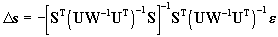
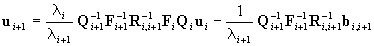
3.2 Reconstruction
Providing that a point is observed in at least two significant
frames, its coordinates can be reconstructed. Let X be such a point,
let x be the sought vector of its coordinates in (O,x,y,z),
and let ui=(ui,vi,1)T
represent Xi, the image of X, in (Zi,ui,vi).
Theoretically, X should lie on all the lines oi
+ liRiFiQiui
simultaneously. If noise is present, X will not lie on the lines
exactly. We measure the distances between X and the lines and minimise
the sum of their squares, i.e., we carry out
 . .
|
(15)
|
The computation yields the result
 , ,
|
(16)
|
where
 . .
|
(17)
|
3.3 Detection of points of interest
The points of interest extracted from the frames both
for calibration and for reconstruction are corners. The corners abound
in the images of both natural and man-made scenes. They often correspond
to the corners of three-dimensional objects and can be unambiguously localised
in the frames. For detecting the corners, we use the Beaudet corner detector
[2].
In 1978, P. R. Beaudet proposed the first corner
detector which works directly with image intensity. The Beaudet detector
locates the corners in an image at local maxima of the Gauss curvature.
Firstly, Beaudets algorithm applies the operator called DET to the whole
image. In this way, we obtain the image in which we search for the local
maxima. The operator DET has the local maxima at positions where the corner
points are situated. The maxima should be greater than a certain threshold.
The operator DET is very simple and can be written as follows
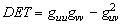 , ,
|
(18)
|
where g=g(u,v) is the input image which is represented
by a two-dimensional function that describes the image intensity and guu,
gvv,
guv
are the partial derivatives. Figure 3 shows an example of the points of
interest detected in an image.
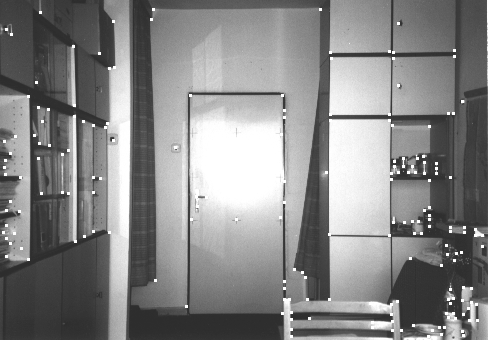
Figure 3. Points of interest detected in an image.
3.4 Tracking the points of interest
Once a point of interest is detected in a frame, it
is tracked in the subsequent frames, i.e., in the subsequent frames, we
seek for the images of the same point of the scene. For tracking, we use
all the frames produced by the camera, i.e., not only the significant frames.
In this section, therefore, by 1,2,...,n we mean the indices in
the sequence of all frames. Let ui-k,...,ui
be the coordinates of the images of a point X in the frames Ii-k,...,Ii
(k>0). The task of finding the coordinates ui+1
in Ii+1 of the image of
X will be easier if some estimation u*i+1
of ui+1
is available. We use the Kalman filter for this purpose. Recall that in
Kalman filtering, the system model, which describes the expected evolution
of the vector si of state variables
over time, is of the form si+1=
Fi+1,isi+
Didi
+ Gixi.
The model of measurement is zi=
Hisi+hi.
The values si, di,
zi,
xi,
hi
are the state vector, deterministic input, vector of measured values, process
noise and measurement noise, respectively. In order to determine
the system model for tracking the points in the frames we use Eqs.(2),(5).
We obtain
 . .
|
(19)
|
Hence
 . .
|
(20)
|
As can be easily seen, Eq.(20) is of the form that is
expected by the Kalman filter. Its use, however, is not easy. In order
to determine the value of ui+1,
the matrices Qi+1,
Fi+1,
Ri,i+1
and the vector bi,i+1
are needed. These, however, are not known at the time when the value of
ui+1
is to be computed. Therefore, we use an approximate model. The model
is based on the assumption that the acceleration of the move of the points
of interest is constant. We use two separate Kalman filters for the u,v
coordinates of each point. In the following text, we restrict ourselves
to the u-coordinate. The state vector is si=(ui,ui',ui'')T.
The matrices of the filter are of the form
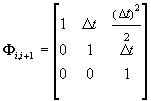 , ,
|
(21)
|
 , ,  , ,
|
(22)
|
where Dt=ti+1
- ti. In our model, Gi
is a diagonal matrix, constant over time, compensating for the difference
between the exact and the approximate model. Note that besides predicting
the coordinates of points in future frames, the Kalman filter is also used
for determining the values of coordinates used for calibration and reconstruction.
The filter reduces the influence of noise and gives the coordinates in
sub-pixel accuracy, which improves the precision achieved in calibration
and reconstruction.
The algorithm for tracking the points of interest
in the sequence of frames will be presented in the following text. Consider
the sequence of frames I1, I2,
...,
In produced by a camera in times t
= 0, 1, ...,
n. The correspondence is a symmetric and transitive
relation between two images of the same point. Finding all corresponding
images of one point is equal to calculating the transitive closure. We
implement the detection of correspondence as finding pairs of corresponding
points in consecutive images It and It+1.
The algorithm we propose solves this task. In time t, we find the
correspondence between the points Xt and Xt+1.
To understand the algorithm correctly, we have to awake that we have already
found the point Xt in time t-1. In time
t-1,
this point was needed for finding the correspondence with the point Xt-1.
The detailed description of the algorithm for finding the correspondence
follows. We will describe the steps that are executed for every frame taken
in time
t. The algorithm consists of three sections, denoted by
A, B, C.
A. Preparing the image It+1.
(1) We prepare the image It+1
for next processing. The image is read from a file produced by a camera
or taken by any other form.
(2) In the image It+1,
we find all the points of interest. The points of interest are detected
by one of the corner detectors. Every point found in this way is inserted
into a search array and is denoted by a unique index. The corresponding
points have the same index.
B. Finding the filtered value and prediction
We denote by X¢t
the value corrected by the Kalman filter in time t, and by X*t+1
the prediction provided by the Kalman filter in time t+1.
In this section, the algorithm falls into two parts. If a new point Xt
is found in the frame It, we continue by Step
3. If the point Xt is found as a point that
corresponds to the point Xt-1,
we continue by Step 4.
(3) If a new point is found, we initialise two Kalman
filters. One for the coordinate u and the other for the coordinate
v.
Both the prediction X*t+1
and the filtered value X¢t
are equal to the coordinates of the new point Xt.
(4) We actualise the Kalman filters for both coordinates
u
and v of Xt which has been found as
corresponding to Xt-1.
The filters provide the prediction X*t+1
and the filtered value X¢t
in which the influence of noise is reduced.
C. Finding the point corresponding to Xt
(5) For point Xt, we
determine a vicinity. In this vicinity, we will find the candidates for
correspondence. The vicinity is a circular area whose radius is r
and whose centre lies in the predicted position X*t+1.
We choose the size of r to be inversely proportional to time t
since as t grows, the prediction X*t+1
of the Kalman filter is more accurate. For the size of r, we can
write
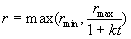 . .
|
(23)
|
If Xt is a new point, we
must choose the size of vicinity large enough to ensure reliably finding
first candidates for correspondence. The starting size of the radius is
rmax.
Later, the size is computed by Eq. (23). The size r is never less
then a minimum rmin. The parameter k
determines how fast the size of vicinity decreases.
(6) All points Y that were found in the vicinity,
are regarded as candidates for correspondence and the correspondence between
Xt
and the candidates is then checked up. In a sequence of frames, there are
usually only small differences between the consequent images, hence we
can say that the image functions in vicinities of corresponding points
are approximately the same. Therefore, we compare the image function of
a current frame in a vicinity of tracked point Xt
with the image function of the consequent frame in vicinities of all candidates
Y.
In practice, we use a rectangle area of size w´
h. Both w and h are set to
appropriate value, the recommended size is 3-9. The vicinities are compared
by a function rel that gives the function values from the interval
0¸1. If the
value of rel is one, the images in both vicinities are the same,
if the value is zero, the images are different. Let ut,
vt
be the coordinates of the tracked point Xt
in time t and let ut+1
and vt+1 be the coordinates
of the candidate Yt+1
in time t+1. Let l
denote one of the colour components. In a colour image, each pixel has
three colour components
r, g, b. We introduce L={r,
g,
b}.
Suppose that the values of the colour components of pixel are chosen from
the interval Jmin¸Jmax.We
defined the function rel as follows
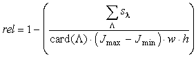 , ,
|
(24)
|
where
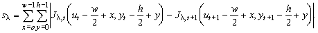
|
(25)
|
The value sl
is a difference of the vicinities of Xt and
Yt+1,
Jl,t
and Jl,
t+1
are the image functions in the particular frames. The function card returns
the number of elements in the set L.
If we know the value of rel for all candidates Y, we choose
the candidate for which the value is considerably greater than for the
others. If the function (24) gives the same value for two or more candidates,
we choose the candidate that is closer to the predicted position X*t+1.
If the value of rel is under a threshold th, we say that
for the tracked point, we cannot find the corresponding counterpart. Otherwise,
the point Yt+1 is declared
to be a point corresponding to Xt and is given
the same index as Xt. The value of th
depends on the number of candidates, denoted by
n. For determining
th,
we propose the following expression
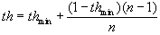 , ,
|
(26)
|
where thmin is a minimum
threshold, which is chosen from the interval 0¸1.
(8) For the radius r of a scanned vicinity,
we introduce an additional condition. If it happened that in Step 6, there
was not found any point of interest in the scanned vicinity, the radius
of vicinity is extended twice and we return back to Step 6 again. At the
same time, the minimum threshold thmin is modified
because we require greater reliability of function rel for candidates.
Therefore, the value of thmin changes according
to the expression
 . .
|
(27)
|
This dependence has been designed by experiments.
(9) If in the search array, any point that was not
classified as corresponding remains, it is regarded as a new point. Every
such point gets a unique index.
After the computation for every image It,
we get an array of indexed points. We can now determine the trajectories
of points for all images Ii , i t.
t.
The above described procedure is heuristic, but our
experiments have shown, that it works well. We tested this procedure on
a certain number of both synthetic and real sequences. Generally, the trajectories
are identified correctly. In some cases, however, certain problems may
occur. It may happen, for example, that the algorithm starts to track a
bad trajectory. Heuristics revealing and correcting these and similar erroneous
situations are implemented. Examples of trajectories that were found in
a real sequence of images are depicted in Figure 4.
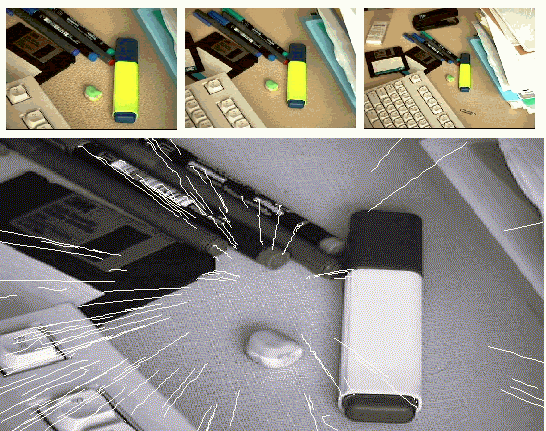
Figure 4. Trajectories of points.
4. Conclusion
In this paper, a method and a computer program for reconstructing
the three-dimensional scenes from the images produced by a moving camera
were presented. A method for calibrating the camera and for reconstructing
the scene from multiple images was proposed, implemented and verified experimentally.
As expected, in comparison with the classical two image approach, the multiimage
approach reduces the sensitivity to noise, which is the key problem in
reconstruction. On the other hand, as the number of significant frames
simultaneously used for calibration increases, the method becomes computationally
expensive. Fortunately, only few significant frames in the time window
(e.g., 3-10 frames) usually suffice to guarantee a good precision of reconstruction.
Although we intended our implementation as an experimental tool and although
we did not aim at constructing a real-time vision system, we are aware
of the fact that the capability to work in real time is important. The
current implementation, however, does not work in real time. The most computationally
expensive proved to be finding and tracking the points of interest. In
calibration and reconstruction, the computational load can be reduced by
processing only an adequate number of significant frames in the time window.
5. References
| [1] |
Sojka, E.: Reconstructing Three-Dimensional Objects
from the Images Produced by a Moving Camera, in Proc. 8thICECGDG,
Austin,
Texas, USA, pp. 160-164,1998. |
| [2] |
Beaudet, P., R.: Rotationally Invariant Image Operators,
in Proc. Fourth Int. Joint Conf. on Pattern Recognition. Tokyo,
pp. 579-583, 1978. |
| [3] |
Daniilidis, K. and Ernst, J.: Active intrinsic calibration
using vanishing points, in Pattern Recognition Letters, Vol. 17,
No. 11, pp. 1179-1189, 1996. |
| [4] |
Ito, M. and Ishii, A.: Range and shape measurement
using three-view stereo analysis, in IEEE Transactions on Pattern Analysis
and Machine Intelligence, Vol. 8, No. 4, pp. 524-532., 1986. |
| [5] |
Longuet-Higgins, H., C.: A computer algorithm for
reconstructing a scene from two projections, in Nature, Vol. 293,
pp. 133-135, 1981. |
| [6] |
Luong, Q., T. and Faugeras, O., D.: Self-calibration
of a moving camera from point correspondences and fundamental matrices,
in International Journal of Computer Vision, Vol. 22, No. 3, pp.
261-289, 1997. |
| [7] |
Bosak, R.: Relative calibration and solving the
calibration equations, Diploma thesis, Technical
University of Ostrava, Czech
Republic, 1998. |