There are many possible surfaces upon which perspective projections can be mapped [GG99]. The most natural one is a sphere centered about the viewpoint. The problem of a spherical projection, is the representation of the surface of the sphere in a form which is suitable for storage and fast access on a computer. This is particularly difficult because a uniform (i.e. equal area for all elements) discrete sampling is desirable. This difficulty is reflected in various distortions which arise in cartography for planar projections of world maps. The mappings which are uniform, allow no systematic access and those which map to a plane distort significantly.
Another possibility is a set of six planar projections in the form of a cube with the projection center in the middle. While this representation can be easily stored and accessed by a computer, it is difficult to achieve the precise camera position and orientation. Also the planar cubic mapping does not represent a uniform sampling, it is considerably oversampled at the edges and corners. It is difficult to avoid artifacts from discontinuities at the image borders.
Therefore a projection on the surface of a cylinder has been suggested. One advantage of the cylinder is, that it can be easily unrolled into a simple planar map, making computer access easy. Another advantage is that a cylindrical panorama can be obtained more easily than a spherical one. Most recording systems support this class of panoramic images. A drawback is the limited vertical field of view.
With a cylindrical panorama two of the three rotational degrees of freedom
can be emulated completely and the third one partly. A full rotation about the
vertical axis is possible. With a rotation about the horizontal axis a limited
view upwards and downwards can be realized. But the vertical field of view can
not be greater than 180
![]() . Therefore a view straight up or down is not possible. A roll motion can
also be simulated, but this rotation of the image is not reasonable, because
this motion is not common in conventional photography. By modifying the field of
view of the artificial camera, a zooming effect can be achieved. But through
this image magnifying no new details can be seen. With bilinear filtering jagged
edges resulting from the limited image resolution can be reduced.
. Therefore a view straight up or down is not possible. A roll motion can
also be simulated, but this rotation of the image is not reasonable, because
this motion is not common in conventional photography. By modifying the field of
view of the artificial camera, a zooming effect can be achieved. But through
this image magnifying no new details can be seen. With bilinear filtering jagged
edges resulting from the limited image resolution can be reduced.
Due to the curved projection surface used when making cylindrical panoramic images strong distortions are inescapable. To generate new views, these distortions have to be corrected. For that purpose the mantle of a cylinder is covered with the panoramic image and viewed through a central projection from the center of the cylinder.
In other systems (e.g. Quicktime VR [Che95])
a custom image warping algorithm has been used for this task. However the goal
of this work is to use the OpenGL graphic system and therefore a standard
rendering pipeline. One can produce arbitrary image distortions by texturing a
uniform polygonal mesh and transforming the vertices appropriately [HS93].
To warp the panoramic image, a cylindrical surface is approximated with a
triangular mesh and the synthetic camera is placed in the center of the cylinder
(Figure 1).
By taking a point in 3-D world coordinates (X,Y,Z) and
mapping this point with a central projection with the center O onto the
surface of a cylinder (see Figure 2) we
get formula (1). This gives the transformation
in cylindrical 2-D coordinates
![]() [SS97].
[SS97].
![]() corresponds to
the rotation angle and
corresponds to
the rotation angle and ![]() to the scanline. Whereas in the resulting panoramic image
to the scanline. Whereas in the resulting panoramic image ![]() corresponds to the x-coordinate and
corresponds to the x-coordinate and ![]() corresponds to the y-coordinate. The cylinder radius r is equal to
the focal length f.
corresponds to the y-coordinate. The cylinder radius r is equal to
the focal length f.
In order to warp the panorama for viewing, the image is projected from the
cylindric surface to a plane, which is normal to the optical axis and tangents
the mantle at the point H (Figure 3).
A point
![]() on the cylinder mantle is transferred after formula (2)
into a point
PP(xE,yE)
on the plane [Hof99].
on the cylinder mantle is transferred after formula (2)
into a point
PP(xE,yE)
on the plane [Hof99].
The process of warping can now be accomplished by an algorithmic operation,
called warp operation [Che95], [Hof99].
As one sees in Figure 3, the projection
on a plane and following display with a central projection is equivalent to a
direct projection of the mantle points through O (the points lie on the
same ray).
In order to proof that both methods provide the same results, the image plane
coordinates
(xI,yI) from (2)
are transformed with formula (5)
to projective coordinates
![]() .
If these points are seen under a central projection (O,d) this
gives (6).
.
If these points are seen under a central projection (O,d) this
gives (6).
As expected, both methods provide the same result:
![]() . Now it
remains to be seen, that every warped view generated from the distorted
panoramic image data is actually a central projection.
. Now it
remains to be seen, that every warped view generated from the distorted
panoramic image data is actually a central projection.
Inserting of formula (1) in (2) gives the central projection in formula (7). The rendering of the undistorted view gives in fact the same picture that a normal camera would take.
The polygon mesh, whose shape was derived in the previous section, has to be
textured with the panoramic image. This leads to the following problem: the
panoramic image can be very big (e.g.
![]() Pixel).
The rendering hardware however can only work with small sized textures. Thus the
input data has to be divided into suitable parts. These parts are sent as single
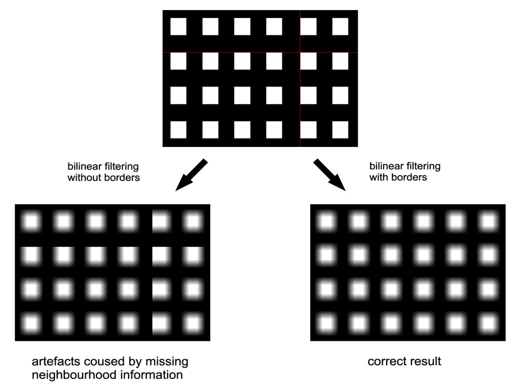
textures to the hardware. If bilinear filtering is used, new problems occur at
the texture border. In bilinear filtering [SA99,
S. 125ff] the weighted median of the color of the four nearest pixels is
calculated. At the texture border these neighborhood values are not
accessible.This results in filtering artifacts. Figure 4
shows a magnified cutting from a synthetic test image. The artifacts caused by
incorrect filtering are clearly visible. There are two possibilities to support
neighborhood data:
Pixel).
The rendering hardware however can only work with small sized textures. Thus the
input data has to be divided into suitable parts. These parts are sent as single
textures to the hardware. If bilinear filtering is used, new problems occur at
the texture border. In bilinear filtering [SA99,
S. 125ff] the weighted median of the color of the four nearest pixels is
calculated. At the texture border these neighborhood values are not
accessible.This results in filtering artifacts. Figure 4
shows a magnified cutting from a synthetic test image. The artifacts caused by
incorrect filtering are clearly visible. There are two possibilities to support
neighborhood data:
By using the texture matrix for modifying texture coordinates, switching between hardware texture border and software texture border is easy. When using the former method the texture matrix must be the identity matrix.
Memory management is another important aspect, because texture data can reach a size of 50 MByte or more. To achieve good efficiency the implementation uses OpenGL texture objects [SA99, S. 132ff]. The texture objects are handled stand-alone from OpenGL with a priority system. If all texture objects have the same priority most of the OpenGL implementations apply a last recently used strategy. This means currently used texture objects remain resident, unused texture objects are swapped out to less efficient memory areas. That is sufficient to achieve good response times. Moreover by using specific prioritizing improvements are eventually possible. The OpenGL system tries to hold the texture data (visible image parts) in texture memory. If the user moves the panorama, new texture data has to be loaded and old texture data has to be deleted. This is a time consuming task which leads to noticeable framerate reduction. For systems with unified memory architecture this is not true, they show a constant framerate under all conditions. In these systems the main memory is also used as texture memory, there is no bottleneck transporting data over the system bus.
![\begin{displaymath}{\small T=\left[
\begin{array}[c]{cccc}%
\frac{w-2}{w} & 0 & ...
...1}{h}\\
0 & 0 & 1 & 0\\
0 & 0 & 0 & 1
\end{array}\right] }
%
\end{displaymath}](images/img25.gif)