Functionality

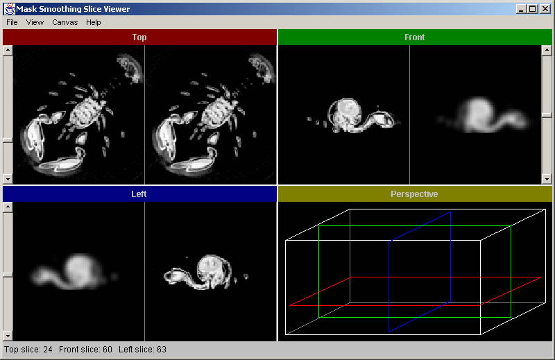
The working area of the application is divided into four parts, three othogonal views and one perspective view, where the relative position of orthogonal views is shown (see the figure 3). But this can be changed in the menu ''View''. In order to see some details only in one orthogonal view, it is possible to switch to this type of view, and it is extended to the whole working area. The orthogonal views consist of two drawing areas to be able to see simultaneously two types of data sets. To move within the slides in one particular direction, the user should move the slider of the scrollbar. This is initialized to a maximal value. The slider size changes after the filtering computation. This effect and also the label in the status bar at the bottom indicates that the computation is finished. The scrollbar range is set to the number of slices in the corresponding direction. This means, one click at the scrollbar button causes that the neighboring slice of the current one will be shown. The change of the viewed slice is immediately visible also in the perspective view and in the status bar, where the number of visible slices is shown. This features make the interaction with the tool user friendly, but this is not the most important property. What makes the tool really powerful is the possibility of choosing and setting various filters for convolution and deconvolution.

Figure 3: Filtering a CT scan of a lobster. Top view shows the original and the filtered data. Front view and left view show the corresponding convoluted and deconvoluted slices respectively.

This is very useful for the algorithm analysis and comparison with already existing methods used for smoothing. There are four categories of filters, where the sum of the weights is 1:

• Basic Cubic Filter - This is the simplest type, it calculates the average value of a cubic voxel neighborhood
• Gaussian Cubic Filter - Gaussian-like filter, where the weigth of a neighboring voxel is the reciprocal of its Manhattan distance from the current voxel.
• Gaussian Spherical Filter - Similar to the previous type, but instead of Manhattan distance an Euclidean distance is calculated.
• Mask Smoothing Filter - Filter kernel of the algorithm we have implemented. The dimensions are . The first three filter types can be modified by changing the filter dimensions and the Mask Smoothing Filter is parametrized by $S$ (smoothing) and $G$ (feature preservation) parameters. This settings can be changed in the Settings dialog in the File menu. There are also some gradient settings in order to improve the results of the feature-preserving algorithm:
  • Threshold - below this value the gradients are considered to be zero.
  • Multiplier - scalar value used for emphasizing the gradient values.
  • Type - central differences or 4D linear regression [3].

Actually only these parameters have to be set before the computation. If the filter is already stored in a file, it is possible to reload it. This can be done by selecting the Open Filter menu item from the File menu. Also the data file has to be loaded analogous with Open Filter but Open Datafile menu item has to be chosen. The computation starts by clicking on the Run menu item in the File menu. When the computation is finished, it is possible to move slice-by-slice within the data set. As already mentioned, it is possible to view two data sets in one direction simultaneously (always the same slice). If one of the first three filter kernels was chosen for the computation, there is a possibility to change the data sets to be shown. For example in the Top view the original and the deconvolved data sets are shown, in the Front view convolved and the deconvolved data sets and original and the convolved data sets. All this can be customized in the Canvas menu. For some error or computational time information, the Statistics menu item from File menu item has to be chosen. It is also possible to save the deconvolved data set into a file. The last menu is Help, where the Online Help and About menu item are available. As it can be seen, this tool gives the user a lot of possibilities for analysis, also looking for the optimal $S$, $G$ and gradient parameters. In the ''slice show'' using one magnified view the user can quickly recognize if some structures are lost (because of smoothing) or not.