Using textures for shading

The solution that yields a result equivalent to the thin tube approach is actually a variant of fake Phong shading applied to lines. The fake Phong method uses the hardware-accelerated texturisation for shading. The idea is to let the graphics library and the hardware transform and linearly interpolate some adequate values, and store the corresponding pre-calculated light intensities in a texture. The texture transformation matrix mechanism allows us to calculate up to three dot products and use them as texture co-ordinates. The simplified shading equation for local lighting is:

$$L = k_{a} + k_{d}\vec{L}\cdot\vec{N} + k_{s}(\vec{R}\cdot\vec{V})^n$$

$k_{a}$, $k_{d}$, and $k_{s}$ are constant coefficients, characterising the material. $\vec{L}$ is the light vector, $\vec{V}$ is the view vector, $\vec{N}$ is the surface normal and L is light intensity or radiance. The reflection vector $\vec{R}$ may be expressed as:

$$\vec{R} = 2\vec{N}(\vec{L}\cdot\vec{N}) - \vec{L}$$

That way the radiance is expressed as a function of $\vec{L}\cdot\vec{N}$ and $\vec{V}\cdot\vec{N}$:

$$L = k_{a} + k_{d}\vec{L}\cdot\vec{N} + k_{s}\Big((2\vec{N}(... ...dot\vec{N})(\vec{L}\cdot\vec{N}) - \vec{L}\cdot\vec{V}\Big)^n$$

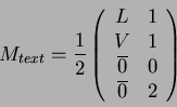
It is possible to use these two values as texture co-ordinates, however, the approximation will not be perfect. Although the interpolation of the dot products is equivalent to the interpolation of the normal vector, there is no possibility to normalise the interpolated vector for every pixel. This method is usually called flat Phong shading. If the normal vector is set as the vertex texture co-ordinate for every vertex, the dot products are evaluated and scaled into the [0,1] domain by the texture transformation itself, provided the transformation matrix is set up as follows:

$$M_{text}=\frac{1}{2}\left( \begin{array}{cc} L & 1\\ V ... ... \overline{0} & 0\\ \overline{0} & 2 \end{array} \right)$$

Unfortunately, it is not possible to completely eliminate the normalisation problem without multiple three-dimensional textures. However, a different approximation is obtained if we do not interpolate the normal itself, but two other vectors perpendicular to each other and the normal, and applying the Pythagorean theorem. If both diffuse and specular lighting are needed, this still requires a huge three-dimensional texture. The method is called fake Phong shading [2], and although it tends to create exaggerated lights in darker areas, it is more accurate than flat Phong shading near the more important highlighted spots.

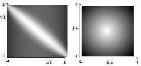
Figure 6: Textures used for illuminated lines[5] and in fake Phong shading[2]. J and K vectors are perpendicular to the surface normal.