Illuminated streamlines

Figure 7: Illuminated streamlines

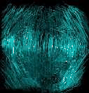How the shading method described above can be applied to lines was described by Zöckler [5]. In the case of lines the normal vector is not unique, and it is of course not sufficient to select an arbitrary one. If the line was a thin tube, intensities for all the possible normal vectors could be visible. It is of course the most intense value that catches the eye, and therefore we have to choose the normal vector corresponding to that value. That vector is the normal coplanar to the light vector $\vec{L}$ and the tangent $\vec{T}$. Luckily, $\vec{L}\cdot\vec{N}$ and $\vec{R}\cdot\vec{N}$ can be expressed using $\vec{L}\cdot\vec{T}$ and $\vec{V}\cdot\vec{T}$:

$$\vec{L}\cdot\vec{N} = \sqrt{1 - (\vec{L}\cdot\vec{T})^2}$$

$$\vec{R}\cdot\vec{N} = (\vec{L}\cdot\vec{T})(\vec{V}\cdot\ve... ...- (\vec{L}\cdot\vec{T})^2} \sqrt{1 - (\vec{V}\cdot\vec{T})^2}$$

Furthermore, if the tangential is interpolated instead of the normal, the inaccuracy of the interpolation becomes less significant. The $\vec{L}\cdot\vec{T}$ and $\vec{V}\cdot\vec{T}$ products will contain some error when the light and the streamline, or the eye vector and the streamline are nearly parallel. This means, that the line should either be dark or barely visible at all. The trick is actually not different from that of fake Phong shading, the dot product is not calculated for the normal, but for a perpendicular vector. However, because of the clever selection of the normal, the three-dimensional texture map is not necessary. If the texture vector associated with the vertices is the tangent vector, the dot products are evaluated via the transformation. The luminance map is filled up according to the radiance formula:

$$L(LT,VT) = k_{a} + k_{d}\sqrt{1 - (\vec{L}\cdot\vec{T})^2} ... ...}\cdot\vec{T})^2} \sqrt{1 - (\vec{V}\cdot\vec{T})^2} \Big)^n$$