Feature-based Volume Rendering of Simulation Data

Matej Mlejnek
mlejnek@cg.tuwien.ac.at

VRVis Research Center
Vienna / Austria
http://www.VRVis.at/vis/

Abstract:

In this paper we present a framework for interactive volume rendering of high-dimensional flow simulation data. Our approach combines information visualization, flow visualization, as well as volume visualization techniques for volumetric flow visualization. Interactive feature specification by use of multiple linked views and composite non-binary brushes enables selection and multiple definition of volumetric features. Further, two-level volume rendering is employed in order to depict the desired flow structures in a focus-plus-context style showing the features in detail, while the remaining data is rendered either semi-transparently or contour-like, allowing the user a full overview of the data set.

Introduction

Recently, volumetric flow visualization of large data sets got one of the most attractive and challenging fields in scientific visualization [18]. However, data acquired from flow simulation comprises not only vector data, but also many scalar data values (e.g., pressure, vorticity, etc.) per sample point. Unfortunately, common flow visualization techniques are based mainly on vector data, taking into account only some of the scalar data attributes. On the other hand, scalar data in 3D can be depicted by volume rendering methods (e.g., iso-surfacing, alpha-compositing). Volume rendering assigns color value to each pixel of the output image. The colors and opacities are interpolated and merged with each other in back-to-front or front-to-back order to yield the resulting color of the pixel. A crucial part of volume rendering is the transfer function, which assigns opacity and color value to each voxel in the data. However, transfer function design has become a research topic on its own [17], the transfer function mapping is limited mostly to one scalar voxel value (or also its first and second derivatives) at each sample point [12]. In addition, this is done mostly (semi-)automatic, without user interaction. In a flow data set a non-interactive approach would fail due to the absence of sharp boundaries. Thus, we employ interactive transfer function design based on specific attributes as well as on the spatial position of features (section 3.2). This paper describes a hybrid approach to volumetric flow visualization, applying volume rendering on flow data segmented in an interactive step. To reduce occlusion problems, we propose an implicit feature-based approach. Interactive information visualization techniques (e.g., brushing in scatterplot), in detail described in section 3.1, are employed to select features (subsets of the data with similar attributes) within a 3D scene. A feature selections can be sorted and saved for further sessions using a feature description language, and rendered in RTVR in a two-level rendering style (section 3.3). Finally, section 4 presents various rendering modes and configurations.

Related Work

The following chapter gives an overview of the most appealing approaches to 3D flow rendering. Crawfis et al. [1] and Ebert et al. [5] introduced volume rendering of flow data obtained from computational simulation of climate and fluid dynamics, respectively, and extended volume rendering algorithms to enable vector and scalar field data representation. Later, Frühauf [6] extended the scalar field ray casting concept to render vector fields with streamline shading at sampling points. Recently, rendering of flow volumes has been further developed for the representation of time-varying data and used in a wide area of computer graphics: Glau [9] used a hardware-assisted system for analysis of computational fluid dynamics, performing a costly resampling step to cartesian grid, necessary for rendering of unstructured grids obtained from simulations. Ebert et al. [4] presented a new concept for non-photorealistic volume illustration of flow data by applying silhouette enhancement on a 3D flow dataset. Swan et al. [19] described a simulation system for computational steering extended to CAVE environment in order to improve the interaction with the rendered model. Ono et al. [15] presented a CAD-based thermal flow visualization system applied in automotive industry. The volume rendering was used to depict the time-dependent temperature values from simulations in an automotive cabin.

Framework

When dealing with volumetric data, due to occlusion and often also due to missing rendering capabilities, it is possible to depict only a small portion of the data simultaneously. Especially if large and high-dimensional data sets are investigated, as ones resulting from computational simulation, the question of what data to display, gets crucial. Feature-based visualization assumes a subset of the original data set to be of special interest (in focus), while the remaining part of the data set is not depicted to avoid visual clutter. A degree-of-interest (DOI) function can be used in order to separate data in focus from context information. According to the user's interest, every sample point is assigned a 1D DOI value, depending on whether the user is interested in that part of the volume or not (1 represents objects of interest, while 0 represents sample points in context). In this work, we utilize a non-discrete DOI function [3] in order to reflect the smooth characteristics of the data acquired from flow simulation. One can define a smooth boundary along a selected feature or an attribute, representing the continuous transition from objects in focus to the context. In other words, a feature with a smooth boundary can be represented by smooth DOI function, i.e., a function that continuously maps the defined "user's interest" to the [0,1] range. In volume visualization, the role of object discrimination is mostly addressed via opacity transfer functions, while the color transfer function enhances the visual perception of displayed objects by shading or by different coloring of objects that belong to different structures (e.g., organs). Unfortunately, the smooth distribution of flow data values along spatial dimensions makes the (semi-) automatic threshold-based segmentation without user interaction quite difficult. Therefore, to define the color and opacity of interesting structures in a large multi-dimensional volume we employ an interactive brushing. 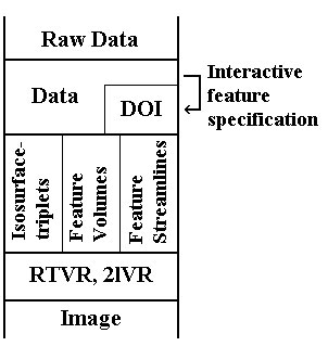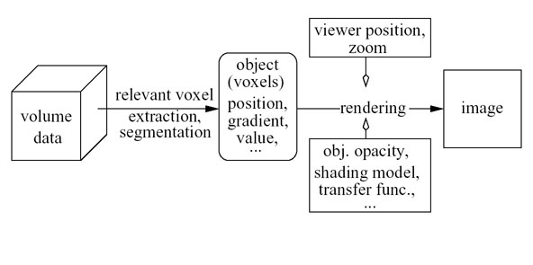In the scope of this work, we divided the visualization mapping from raw data to resulting image into three phases (figure 1). Firstly, the raw data acquired from simulation is segmented according to user's selections in n-dimensional data attribute space, resulting in a smooth DOI function for each selected feature. Then, an appropriate volumetric representation of the selected features has to be chosen. We propose three models for volumetric feature representation: isosurface-triplets, feature volume and feature streamlines. Each of them has its pros and cons depending of the feature's characteristics. Finally, the entire feature set is rendered in two-level rendering style.

**Figure 1:** Feature-based volumetric visualization pipeline.

Interactive feature specification

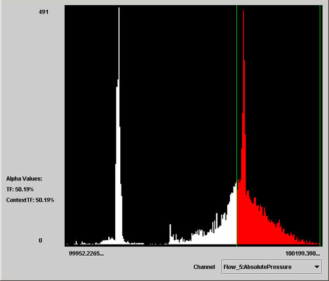
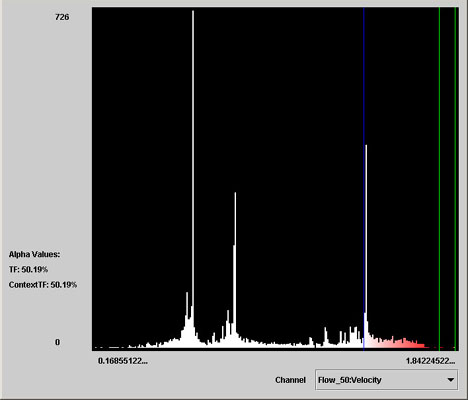
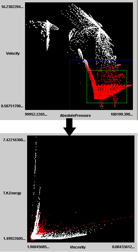
Brushing is a very effective tool, especially when combined with linking. The way how the user defines the features is very intuitive and straightforward even if large high-dimensional data are under investigation. The primary goal of this procedure is to guide the user while brushing in the n-dimensional domain of the simulation data to the desired feature specifications. An arbitrary number of views, depicting one or more data set attributes (e.g., histograms, scatterplots, etc.), are linked, brushing in one window affects visual appearance in all other views. Our framework deals with composite brushes in n-dimensional domain, allowing identification of complex features of interest. Figure 2 demonstrates the concept of linking and brushing: User brushes a smooth selection on a scatterplot which depicts the relationship between absolute presure and velocity data attributes. The selection immediately affects all linked views (e.g., viscosity vs. turbulence kinetic energy) showing what range from the other data attributes is selected. A specific feature can be defined by repeated selection in one or two-dimensional domains of histograms and scatterplots respectively until the desired structure is found.

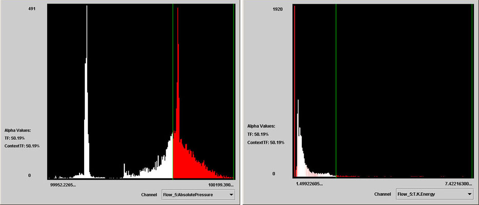
**Figure 2:** Brushing in the first scatterplot affects the selection in the second linked view.

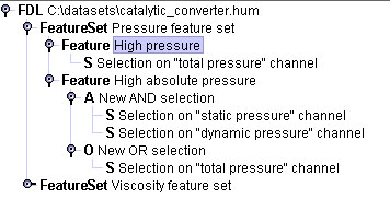
These approximate selections can be refined using sliders or typing numerical values in the allowed range of data attribute. The intermediate result from the interactive feature selection is represented in a compact structure called feature definition language (FDL) [2]. The FDL is closely related to a data set acquired from computational flow simulation. The root layer consists of a filename and an arbitrary number of feature sets (figure 3). A feature set is a group of selected features that are to be shown simultaneously. The user can switch between feature sets, add new ones, delete, or move features from one set to another during the session. A feature layer is composed in a similar way, but consists of one or more feature characteristics, i.e., one or two-dimensional brushings in a histogram or a scatterplot respectively. A feature characteristic, the lowest FDL layer, storing only brushed (smooth) range and the corresponding data attribute, can be logically combined with other feature characteristics allowing n-dimensional feature definitions. If the spatial dimension is taken into account as an additional attribute, feature definition based on spatial position of the feature can be refined.

**Figure 3:** An example of FDL. The root node contains an arbitrary number of feature sets, which can be depicted simultaneously. A feature setc ontains one or more features logically combined of simple selections on data attribute ranges.

Visualization mapping

A smooth DOI function, resulting from multiple brushing in n dimensions, assigns one floating point value between zero and one to every sample point in the investigated object and, thus, identifies the user's degree of interest in each point. This user-defined function has proved to be very useful as an additional attribute in two-level rendering (see section 3). As already mentioned, our framework consists of an arbitrary number of linked views enabling brushing on data attributes and can be grouped into features. Each feature is assigned to exactly one feature set and can be rendered together with other features of the same feature set in the render window. A DOI function, defining the features that belong to a certain features set, can be updated after each feature refinement in the information visualization interface. The DOI function of newly defined and modified features is evaluated in real-time while brushing and used by the volume rendering process after each update. Features which were deleted during the session are removed from the scene and omitted from further investigation process.

Two-level volume rendering with RTVR

Once, the desired features are specified, feature-based volume rendering can be performed. In order to offer the user a variety of object appearance modes, we use two-level volume rendering [10] that combines different rendering techniques for different objects within a 3D scene. Compositing modes can be selected on a per-object basis, giving the user a certain degree of freedom in setting up rendering properties and object attributes. Moreover, clipping in an arbitrary plane can be performed for a single object. For rendering of selected features as well as context information we bring into play RTVR [14], a java-based library for two-level volume rendering of rectilinear volumes at interactive frame rates. In comparison to hardware-based approaches, due to its pure software nature, it provides flexibility and easy extensibility. A fast and memory efficient shear-warp approach implementing a two-level volume rendering metaphor is well-suited also for interactive rendering of large high-dimensional data. When dealing with large time-varying data sets, data, which belong to other time steps, are swapped to the disk. The rendering primitive of RTVR is a voxel. Each voxel is either assigned to a volume object and stored within a special data structure, or omitted from further rendering steps already at segmentation and data extraction phase (figure 4). Segmentation can be done either interactively (see section 3.1), or in a (semi-)automatic way (thresholding, transfer function design, etc.) well-known from medical visualization. Segmentation information can be saved for the use in the next sessions. Since only a small fraction of the original volume belongs to distinct objects of interest, which are to be rendered, a high rendering performance is achieved by significant data reduction. Furthermore, depending on the visualization method of the object, voxels, for example, with low gradient magnitudes or with values bellow the threshold value, are removed.

**Figure 4:** Volume data flow within RTVR (similar to figure 2 in [14].

Due to a highly optimized internal data structure, an RTVR object consists of so called RenderLists containing only object's voxels within one slice. A RenderList is an array of 32-bit structures including 8 bits for each x and y coordinate, therefore, data attributes are restricted only to 16 bits. These are typically split into a 12-bit and a 4-bit field. Transfer function design is based on three look-up tables (1x4bit and 2x12bit) which are available for each object. Of course, this offers many different pros and cons. For instance, shading operations are implemented in a 12-bit LUT taking a voxel's gradient vector as input. The output is used for the RGB color lookup in another 12-bit lookup table. Splitting into two sequentially performed processes speeds up the refresh of LUTs, when only one table has to be updated (e.g., after change of viewer position, only shading table has to be changed). Due to a relative small size of a LUT, this can be done interactively in every frame. For example, if the user chooses another shading model, only the shading LUT has to be replaced. Unfortunately, if the shaded object is to be shown, 12 bits of the voxel's attribute are reserved for gradient information leaving only 4 bits for the remaining attributes (e.g., object opacity information).

Feature-based 3D Flow Visualization

Each feature, defined by a DOI function, corresponds to exactly one volumetric object. The object's appearance can be set up individually for each object, based on the DOI function values of the features sample point as well as derived from any of the attributes of the flow data set (e.g., velocity, vorticity, pressure, etc.). As already discussed, in addition to existing volume rendering modes in RTVR, we propose several new object appearance modes, refined by a DOI function attribute and derived from user's feature specifications in linked views. In the scope of this paper we mainly distinguish between features (objects in context) and the remaining data (context information). In the following sub-sections we propose three main classes of objects, which can be chosen to depict a feature, while object contours or a semi-transparent surface proved to be well-suited for context information. The results are demonstrated on volumetric data sets coming from simulations in automotive industry.

Isosurface-triplet

Iso-surfacing is a fast method often applied with volume visualization due to its simple definition. An iso-surface is fully described by an iso- and an opacity value. To depict the smooth nature of flow data, we propose isosurface-triplet, a volumetric object containing one main iso-surface and an arbitrary number of additional surfaces, which illustrate the desired data attribute inside of a feature or closely surrounding the interesting region. The number of surfaces should be chosen carefully, since a high number can cause visual clutter in the displayed view. An isosurface-triplet's main surface, similar to an iso-surface, is defined by an iso- and opacity value. Additional surfaces are determined by the relative distance from the main surface as well as by relative opacity regarding the opacity of the main surface. The color can be defined for each surface separately. Gerstner [7] presented the use of multiple iso-surfaces for medical data using a multiresolution technique for surface extraction. He assumed value-histogram minimas to be appropriate iso-values for surface extraction. In a case study [8], he demonstrates the approach on data sets from meteorology. Recently, the research of fast extraction of salient iso-values got very challenging [16,20]. Our definition of a isosurface-triplet deals with a very intuitive model depicting the main (middle) surface in green, the inner and outer surface(s) red and blue respectively. The iso-surfaces' opacities depend strongly on the shape and spatial position of the features as well as on the specific goal of the visualization process. Initially they are displayed semi-transparently. 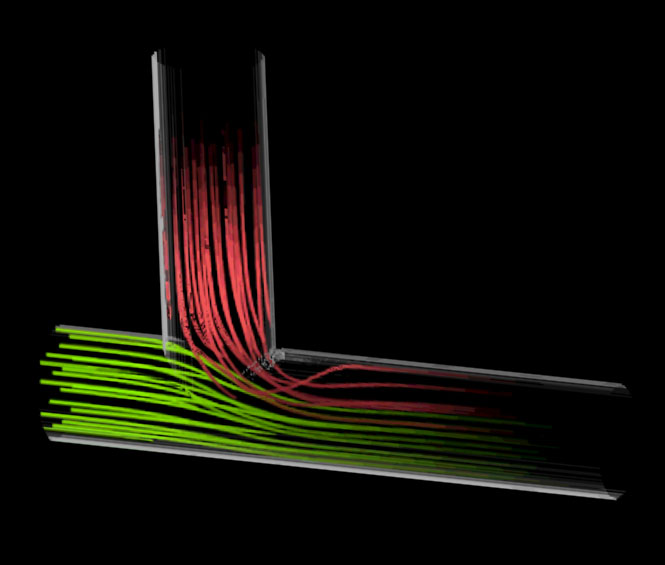Figure 5 shows volumetric data sets coming from simulation in automotive industry. An isosurface-triplet is used to depict the velocity in a region of two joining flows.

**Figure 5:** Isosurface-triplet of velocity of two joining flows. Two inputs (top and left) with low velocity are joining into one fast output.

After investigation of many various feature definitions and shapes, three and five different semi-transparent iso-surfaces proved to be enough for a clear representation of the feature structure. Rendering more than five semi-transparent surfaces simultaneously leads to incorrect color interpretation, while showing more than seven surfaces can hide the feature behind the redundant context objects. The isosurface-triplet is also very useful for depicting of DOI functions even if a feature is defined as a combination of brushes on many different data attributes. Figure 6 depicts a DOI function of a complex feature in spatial coordinates. Red surface localizes an area of focal interest (DOI function = 1), while the areas with 75% and 50% interest are depicted green and blue, respectively.

**Figure 6:** Multiple iso-surfacing of a DOI function, depicting the region of full interest red. The green and blue iso-surface areas are with 75% and 50% interest respectively.

Feature Volumes

**Figure 7:** Feature volume showing the region with high viscosity. The shading of the object improves the spatial perception, while the opacity depicts the DOI function.

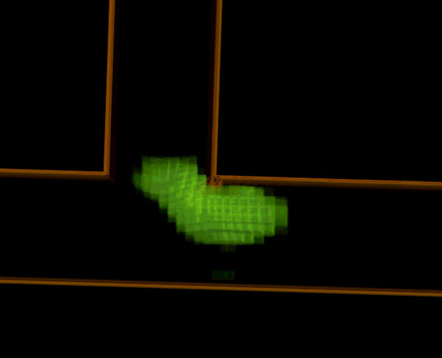
A second group of object representations offers a volumetric representation of the structure(s) of interest. Voxels in areas with non-zero DOI function belonging to one feature are depicted as a volumetric object. In previous work [3], using a DOI function for opacity modulation proved to be appropriate for this kind of visualization. The opacity of each voxel is computed by a linear ramp from its smooth DOI-value. Object's color can be determined in two ways. Firstly, a unique color is assigned to each object to improve its visual discrimination, while color intensity is used for shading (figure 7).

**Figure 8:** Feature with high static pressure. The color identifies the feature in a unique way, while the color intensity depicts the velocity in this area.

Secondly, color intensity can depict another arbitrary data attribute from the data set. Figure 8 depicts a feature with high static pressure. The unambiguousness of the object is achieved by its unique color, while the color intensity represents an additional data attribute. Figure 9 shows a feature volume with both color intensity and opacity depicting the velocity. This color mapping proved to be very useful, particularly if drastically modifying the feature specifications. Investigation of numerous non-colored objects can lead to ambiguous representation of unequal features.

**Figure 9:** Feature volume depicts a feature with high velocity. The color identifies the object, while both color intensity and opacity map the velocity data attribute.

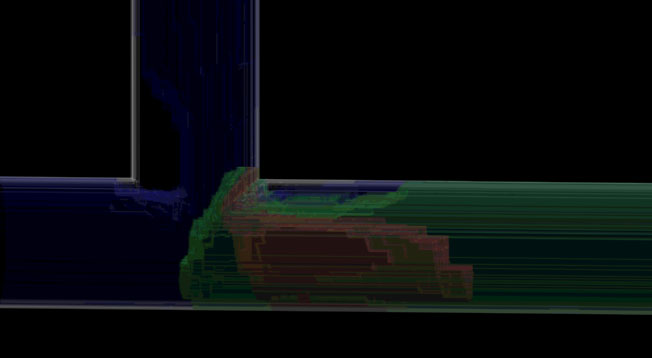
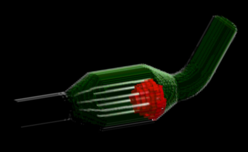
Further, an arbitrary number of feature objects can be composited into one scene in a two-level rendering manner. The object's appearance can be defined on a per-object basis, i.e., each feature is set up individually, choosing the most suitable object attributes related to the feature, which the object represents. Figure 10 depicts two different feature volumes. The region with low velocity (green) is displayed as a shaded object with semi-transparent boundaries, resulted from smooth boundary definition in feature specification step. The region with high turbulence kinetic energy (TKE) (red) is also depicted with semi-transparent boundaries. In this case, the semi-transparency is caused by the TKE data attribute, which is mapped as opacity.

**Figure 10:** The visualization scene consisting of two volumetric features: The green region depicts the area with low velocity with the semi-transparent area along the object caused by smooth brushing. The red region corresponds to an area with high turbulence kinetic energy(TKE); the opacity corresponds to the TKE data value, showing the lower values more transparent. The context is depicted by a surface.

Feature objects, derived from DOI function, can be combined with volumetric object not defined by the user in the brushing step, i.e., objects which are not created directly from DOI function. For example, a surface, designed by thresholding with a low iso-value on one data set attribute, can depict the context information, even if only its contours are displayed (figure 10).

Feature streamlines

The last group of objects useful for feature-based volume rendering with a user-defined DOI function was inspired by Jobard et al. [11]. They introduced evenly-spaced streamline placement, controlling the seeding as well as separating distance between adjacent streamlines. We extended their work to 3D applying a smooth DOI function in order to influence the seeding and breaking of the streamline computation (figure 11). The use of smooth DOI function offers several streamline placement modes that enable the user an intuitive seeding area definition by brushing in the information visualization views.

**Figure 11:** DOI forward streamline computation. Seeding points are positioned in the region of focal interest (red). The DOI function is mapped to object's color intensity; the region with non-zero DOI function is inside of the light-green surface.

Firstly, the seeding of streamline starting points is allowed only in regions with DOI function equal to one (regions of focal interest). This restriction is closely coupled to the style how the region of interest is selected. In this case, it is possible to define desired seed locations rather precisely even by typing numerical values (see: section 3.1). The streamline computation is repeated while the streamline endpoint is situated within a non-zero DOI region, or until it leaves the scene. In the second case DOI values are mapped to color or opacity. Of course, both above mentioned approaches produce similar results, since sample points with zero DOI are displayed either transparent (due to zero opacity) or black (due to zero color). Furthermore, seeding points can be positioned either randomly to speed up the computation, or the seeding condition can be evaluated in every point. Latter enables highest possible seeding density and ensures picking of equal seeding point positions after each update without seeding region modification. Secondly, the seed position is chosen by randomly sampling a probability seeding function used by Löffelman et al. [13]. Comparison of a random floating number 0<n<1 with the smooth DOI function (with the same range) in a random spatial location determines whether the location can be used for seeding. The break of streamline computation is handled similar to previous case. Applying previous schemes in our framework, non-random seeding proved to be more useful allowing the user more explicit investigation of visual changes caused by focus variation due to absence of influence of random entities. A feature is identified by the feature streamline's color in a unique way. The color intensity can be mapped either from the DOI value (figure 12) or the streamline can be shaded using the shading model proposed by Zöckler [21] (figure 11).

**Figure 12:** Two joining feature streamlines. Color intensity is straight proportional to the DOI function. Therefore the streamline in areas of focal interest is depicted brighter than in the area with DOI value below one.

Conclusions and Future Work

We presented an interactive framework for focus-and-context volumetric visualization for data acquired from computational simulations. To reduce occlusion problems, we have chosen a feature-based approach. Features defined in as interactive step can be depicted in three different modes: Isosurface-triplet, Feature volume, or Feature streamline. What representation is to be used for a certain feature, strongly depends on the feature's characteristics and spatial position. The next step to further develop our visualization framework is to extend it to time-varying data. This includes new feature specification techniques also involving new volume rendering modes. Moreover, the need for high quality rendering could require implementation in hardware as well as new simulation techniques yielding more precise data measured on huge number of sample points. But the latter is far behind the scope of this paper.

Acknowledgements

This work has been carried out as part of the basic research on visualization at the VRVis Research Center in Vienna, Austria (http://www.VRVis.at/vis/), which is partly funded by an Austrian research program called Kplus. All data presented in this paper are courtesy of AVL List GmbH, Graz, Austia. A special gratitude goes to Helwig Hauser for helping to prepare this paper, and Martin Gasser, Helmut Doleisch and Markus Hadwiger for implementation of feature specification layer as well as the underlying mesh-library system. Also author would like to thank Lukas Mroz for the implementation of Real-Time Volume Rendering library.

Bibliography

1: Roger Crawfis, Nelson Max, Barry Beccker, and Brian Cabral.
Volume rendering of 3D scalar and vector fields at LLNL.
In Proceedings, Supercomputing '93: Portland, Oregon, November 15-19, 1993, pages 570-576, 1109 Spring Street, Suite 300, Silver Spring, MD 20910, USA, 1993. IEEE Computer Society Press.
2: Helmut Doleisch, Martin Gasser, and Helwig Hauser.
Interactive feature specification for focus+context visualization of complex simulation data.
In Proceedings of the 5th Joint IEEE TCVG EUROGRAPHICS Symposium on Visualizatation (VisSym 2003), to appear, Grenoble, France, May 26-28 2003.
3: Helmut Doleisch and Helwig Hauser.
Smooth brushing for focus+context visualization of simulation data in 3D.
In Journal of WSCG, volume 10, 2002.
4: David Ebert and Penny Rheingans.
Volume illustration: non-photorealistic rendering of volume models.
In IEEE Visualization '00 (VIS '00), pages 195-202, Washington - Brussels - Tokyo, October 2000. IEEE.
5: David S. Ebert, Roni Yagel, Jim Scott, and Yair Kurzion.
Volume rendering methods for computational fluid dynamics visualization.
In Proceedings of the Conference on Visualization, pages 232-239, Los Alamitos, CA, USA, October 1994. IEEE Computer Society Press.
6: Thomas Frühauf.
Raycasting vector fields.
In Proceedings of the Conference on Visualization, pages 115-120, Los Alamitos, October 27-November 1 1996. IEEE.
7: Thomas Gerstner.
Multiresolution Extraction and Rendering of Transparent Isosurfaces.
Computers & Graphics, 26(2):219-228, 2002.
(shortened version in Data Visualization '01, D.S. Ebert, J.M. Favre and R. Peikert (eds.), pp. 35-44, Spinger, 2001, also as SFB 256 report 40, Univ. Bonn, 2000).
8: Thomas Gerstner, Dirk Meetschen, Susanne Crewell, Michael Griebel, and Clemens Simmer.
A case study on multiresolution visualization of local rainfall from weather radar measurements.
In Proceedings of the conference on Visualization '02, pages 533-536. IEEE Press, 2002.
9: Thomas Glau.
Exploring instationary fluid flows by interactive volume movies.
In Data Visualization '99, Eurographics, pages 277-283. Springer-Verlag Wien, May 1999.
10: Helwig Hauser, Lukas Mroz, Gian-Italo Bischi, and M. Eduard Gröller.
Two-level volume rendering - fusing MIP and DVR.
In IEEE Visualization '00 (VIS '00), pages 211-218, Washington - Brussels - Tokyo, October 2000. IEEE.
11: Bruno Jobard and Wilfrid Lefer.
Creating evenly-spaced streamlines of arbitrary density.
In Visualization in Scientific Computing '97. Proceedings of the Eurographics Workshop in Boulogne-sur-Mer, France, pages 43-56, Wien, New York, 1997. Eurographics, Springer Verlag.
12: Joe Kniss, Gordon Kindlmann, and Charles Hansen.
Interactive volume rendering using multi-dimensional transfer functions and direct manipulation widgets.
In IEEE Visualization '01 (VIS '01), pages 255-262, Washington - Brussels - Tokyo, October 2001. IEEE.
13: Helwig Löffelmann and M. Eduard Gröller.
Enhancing the visualization of characteristic structures in dynamical systems.
In Visualization in Sientific Computing '98, Eurographics, pages 59-68. Springer-Verlag Wien New York, 1998.
14: Lukas Mroz and Helwig Hauser.
RTVR - a flexible java library for interactive volume rendering.
In IEEE Visualization '01 (VIS '01), pages 279-286, Washington - Brussels - Tokyo, October 2001. IEEE.
15: Kenji Ono, Hideki Matsumoto, and Ryutaro Himeno.
Visualization of thermal flows in an automotive cabin with volume rendering method.
In Proceedings of the Joint Eurographics - IEEE TCVG Symposium on Visualizatation (VisSym-01), pages 301-308, Wien, Austria, May 28-30 2001. Springer-Verlag.
16: Vladimir Pekar, Rafael Wiemker, and Daniel Hempel.
Fast detection of meaningful isosurfaces for volume data visualization.
In IEEE Visualization '01 (VIS '01), pages 223-230, Washington - Brussels - Tokyo, October 2001. IEEE.
17: Hanspeter Pfister, Bill Lorensen, Chandrajit Bajaj, Gordon Kindlmann, Will Schroeder, Lisa Sobierajski Avila, Ken Martin, Raghu Machiraju, and Jinho Lee.
Visualization viewpoints: The transfer function bake-off.
IEEE Computer Graphics and Applications, 21(3):16-23, MayJune 2001.
18: Frits Post, Benjamin Vrolijk, Helwig Hauser, Robert S. Laramee, and Helmut Doleisch.
Feature extraction and visualization of flow fields.
In Eurographics 2002 State-of-the-Art Reports, pages 69-100. The Eurographics Association, Saarbrücken Germany, 2-6 September 2002.
19: J. Edward Swan, II., Marco Lanzagorta, Doug Maxwell, Eddy Kuo, Jeff Uhlmann, Wendell Anderson, Haw-Jye Shyu, and William Smith.
A computational steering system for studying microwave interactions with missile bodies.
In IEEE Visualization '00 (VIS '00), pages 441-444, Washington - Brussels - Tokyo, October 2000. IEEE.
20: Shivaraj Tenginakai, Jinho Lee, and Raghu Machiraju.
Salient iso-surface detection with model-independent statistical signatures.
In IEEE Visualization '01 (VIS '01), pages 231-238, Washington - Brussels - Tokyo, October 2001. IEEE.
21: Malte Zöckler, Detlev Stalling, and Hans-Christian Hege.
Interactive visualization of 3D-vector fields using illuminated streamlines.
In Proceedings of IEEE Visualization '96, San Francisco, pages 107-113, October 1996.