Kaiser Window

The Kaiser window [6] has an adjustable parameter $\alpha$ which controls how quickly it approaches zero at the edges. It is defined by

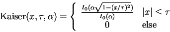$$\textrm{Kaiser}(x,\tau,\alpha)=\left \{ \begin{array}{cl} \... ...rt x\vert\leq \tau \\ 0 & \textrm{else} \end{array} \right.$$ (13)

where I₀(x) is the zeroth order modified Bessel function (for a definition, and a more detailed discussion, of the Bessel functions see, for instance, the Numerical Recipes in C [17]. The higher $\alpha$ the narrower gets the window and therefore, due to the not so severe truncation then, the less severe are the bumps above $\pi$. In Fig. 2 again, but in the fourth row, several Kaiser windows are depicted with different values for $\alpha$. The frequency responses on the right shows that the parameter $\alpha$ directly controls its shape.

Goss [4] used this window to obtain an adjustable gradient filter, but he used it only on sample points so that, in between sample points, some kind of interpolation has to be performed, which he does not state explicitly. In this work, the Kaiser windowed cosc function will be used to reconstruct gradients at arbitrary positions which is, of course, more costly.